下面对目前所有相位恢复的代码进行整理,详细说明每段代码的原理和功能。
使用 PhaseRetrival 工具包进行相位恢复 验证传播函数正确性 下面是使用 PhaseRetrival 工具包进行相位恢复前的准备工作,使用FECO导出的数据(幅值+相位)模拟衍射,以验证衍射部分代码的正确性。
1 2 3 4 5 6 7 8 9 10 11 12 13 14 15 16 17 18 19 20 21 22 23 24 25 26 27 28 29 30 31 32 addpath('E:\组会\其他\实验室历史文件\code\phasepack-matlab-master\solvers' ); addpath('E:\组会\其他\实验室历史文件\code\phasepack-matlab-master\util' ); addpath('E:\组会\其他\实验室历史文件\code\phasepack-matlab-master\initializers' ); global numrows numcols num_fourier_masks masks padding lamda dx;f = 1.65e9 ; lamda = physconst('lightspeed' ) / f; k0 = 2 * pi / lamda; dtheta = pi / 180 ; dphi = pi / 180 ; theta = -pi / 2 :dtheta:pi / 2 ; phi = 0 :dphi:pi ; NF_data1 = 'E:\组会\其他\实验室历史文件\code\phase retrival\NFdata\DATAyyq\l_6lamb_n_97_2-5lamb.efe' ; NF_data2 = 'E:\组会\其他\实验室历史文件\code\phase retrival\NFdata\DATAyyq\l_6lamb_n_97_3-0lamb.efe' ; NF_data3 = 'E:\组会\其他\实验室历史文件\code\phase retrival\NFdata\DATAyyq\l_6lamb_n_97_3-5lamb.efe' ; [Ex1, Ey1, xd1, yd1] = load_NF(NF_data1); [Ex2, Ey2, xd2, yd2] = load_NF(NF_data2); [Ex3, Ey3, xd3, yd3] = load_NF(NF_data3); Ey1_1D = Ey1(:); Ey2_1D = Ey2(:); Ey3_1D = Ey3(:); M = length (xd2); N = length (yd2); dx = (xd2(2 ) - xd2(1 )); dy = (yd2(2 ) - yd2(1 ));
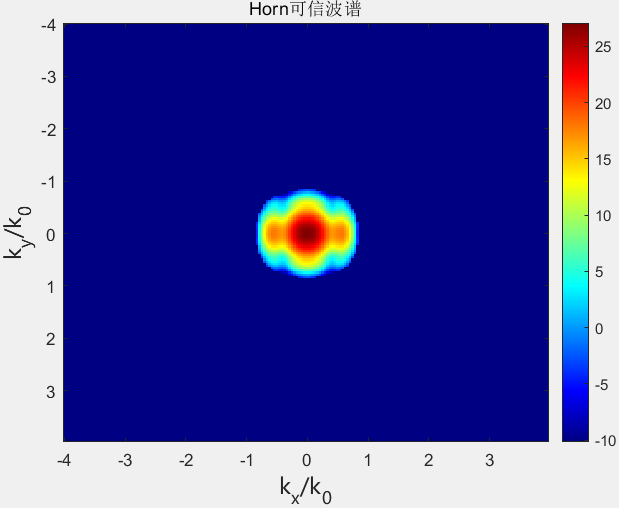
1 2 3 4 5 6 7 8 9 10 11 12 13 14 15 16 padding = 2 ; MI = padding * M; NI = padding * N; m = -MI / 2 :1 :MI / 2 - 1 ; n = -NI / 2 :1 :NI / 2 - 1 ; k_X_Rectangular = 2 * pi * m / (MI * dx); k_Y_Rectangular = 2 * pi * n / (NI * dy); dk_X = k_X_Rectangular(2 ) - k_X_Rectangular(1 ); dk_Y = k_Y_Rectangular(2 ) - k_Y_Rectangular(1 ); [k_Y_Rectangular_Grid, k_X_Rectangular_Grid] = meshgrid (k_Y_Rectangular, k_X_Rectangular); fy1 = fftshift(ifft2(Ey2, MI, NI) * MI * NI) * dx * dy; fy_Magnitude = 20 * log10 (abs (fy1));
1 2 3 4 5 6 7 8 9 10 11 12 13 14 15 16 17 18 19 20 21 22 23 24 25 26 27 28 29 30 31 32 33 34 35 36 kz = sqrt (k0 ^ 2 - k_X_Rectangular_Grid .^ 2 - k_Y_Rectangular_Grid .^ 2 ); W = 0.55 ; H = 0.428 ; w = dx * (M - 1 ); h = dy * (N - 1 ); z0 = 2.5 * lamda; z1 = 3.0 * lamda; z2 = 3.5 * lamda; Reliable_rate = 1 ; thetax_sure = Reliable_rate * atan (0.5 * (w - W) / z1); thetay_sure = Reliable_rate * atan (0.5 * (h - H) / z1); UR = zeros (MI, NI); for i = 1 :MI for j = 1 :NI if ((k_X_Rectangular(i ) * k_X_Rectangular(i ) / ((k0 * sin (thetax_sure)) ^ 2 )) + (k_Y_Rectangular(j ) * k_Y_Rectangular(j ) / (k0 ^ 2 )) < 1.0 && (k_X_Rectangular(i ) * k_X_Rectangular(i ) / (k0 ^ 2 )) + (k_Y_Rectangular(j ) * k_Y_Rectangular(j ) / ((k0 * sin (thetay_sure)) ^ 2 )) < 1.0 ) UR(i , j ) = 1 ; else UR(i , j ) = 0 ; end end end fy_H_Magnitude = 20 * log10 (abs (fy1 .* UR));
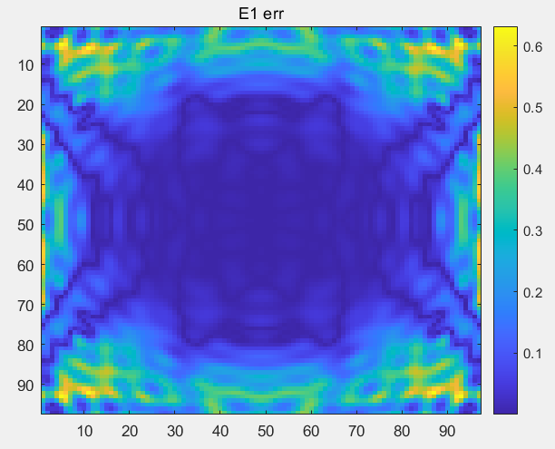
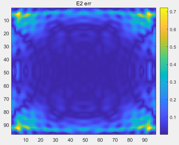
1 2 3 4 5 6 7 8 9 10 11 12 13 14 15 16 17 18 19 20 21 22 23 [numrows, numcols] = size (k_Y_Rectangular_Grid); num_fourier_masks = 2 ; masks = zeros (numrows, numcols, num_fourier_masks); dz = [0 0.5 ]; isim = imag (kz) ~= 0 ; kz(isim) = -1 * kz(isim); for i = 1 :num_fourier_masks masks(:, :, i ) = UR .* exp (-1 i * kz * dz(i ) * lamda); end fy0 = fftshift(ifft2(Ey2, MI, NI) * MI * NI) * dx * dy; x = fy0(:); b_cal = abs (A(x)); b_real = [abs (Ey2_1D); abs (Ey3_1D)];
1 2 3 4 5 6 7 b_err_1 = sqrt (sum(abs (abs (b_real) - b_cal) .^ 2 , 'all' ) / sum(b_cal .^ 2 , 'all' )); b_err_2 = abs ((b_real - b_cal) ./ b_cal); b_err = reshape (b_err_2, [numrows / padding, numcols / padding, num_fourier_masks]); E1_err = (squeeze (b_err(:, :, 1 ))); E2_err = (squeeze (b_err(:, :, 2 )));
PhaseRetrival 工具包进行相位恢复 上面已经验证了衍射过程的正确,下面开始使用 PhaseRetrival 工具包进行相位恢复,这个过程是已经集成好的,只需要设置少量参数即可。
1 2 3 4 5 6 7 8 9 10 11 12 13 14 15 16 17 18 19 20 21 22 23 24 opts = struct; opts.algorithm = 'RAF' ; opts.initMethod = 'Weighted' ; opts.tol = 1e-6 ; opts.verbose = 1 ; opts.maxIters = 1000 ; fprintf('Running.....\n 算法: %s \n 初始化: %s \n 误差: %s \n 迭代次数: %d \n' , opts.algorithm, opts.initMethod, opts.tol, opts.maxIters); [x, outs, opts] = solvePhaseRetrieval(@A, @At, b_real, numel (k_Y_Rectangular_Grid), opts); recovered_image = reshape (x, numrows, numcols); fprintf('Image recovery required %d iterations (%f secs)\n' , outs.iterationCount, outs.solveTimes(end )); by_retrival = A(recovered_image); by_retrival = reshape (by_retrival, [numrows / padding, numcols / padding, num_fourier_masks]); E2 = (squeeze (by_retrival(:, :, 1 )));
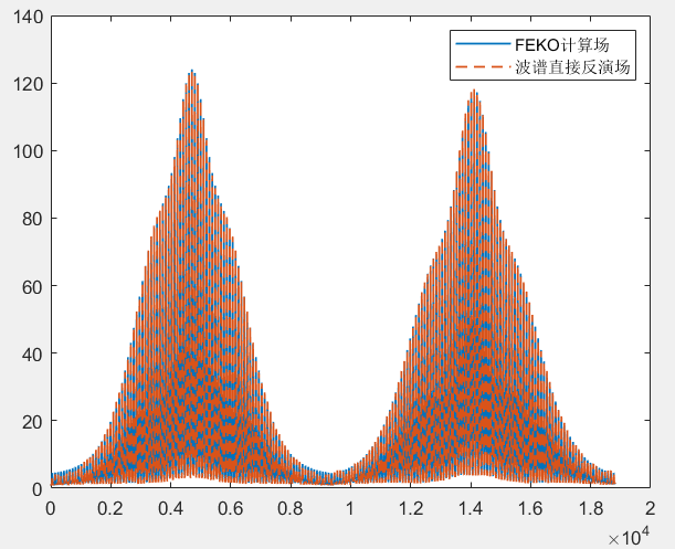
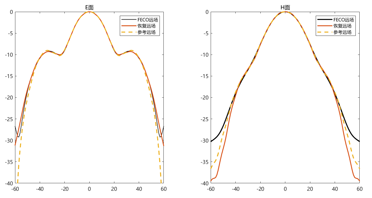
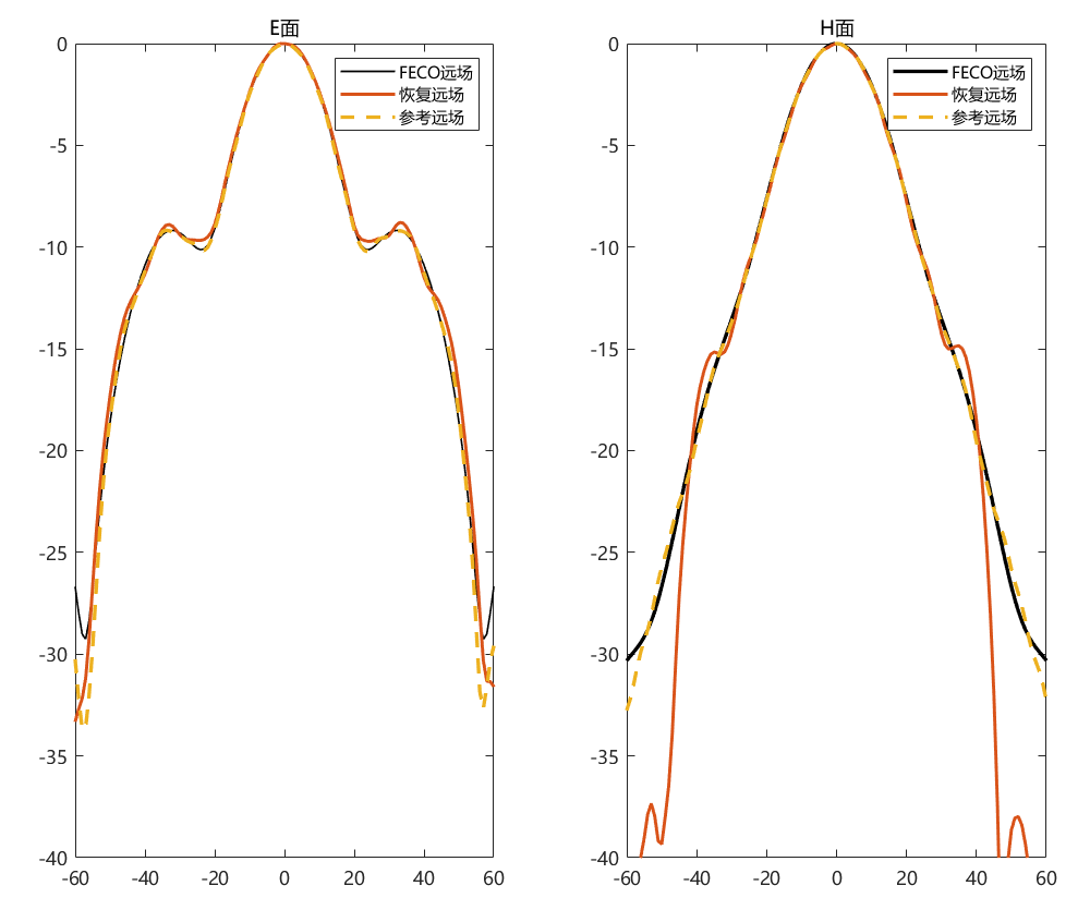
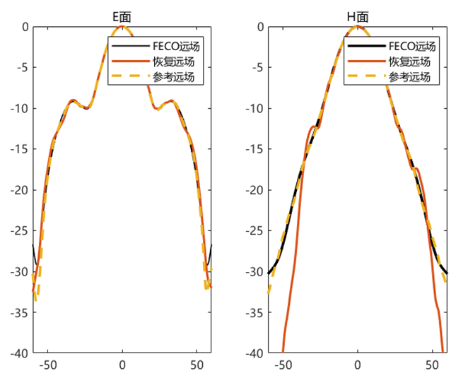
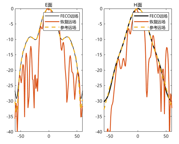
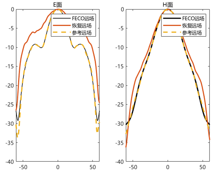
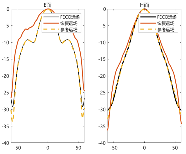
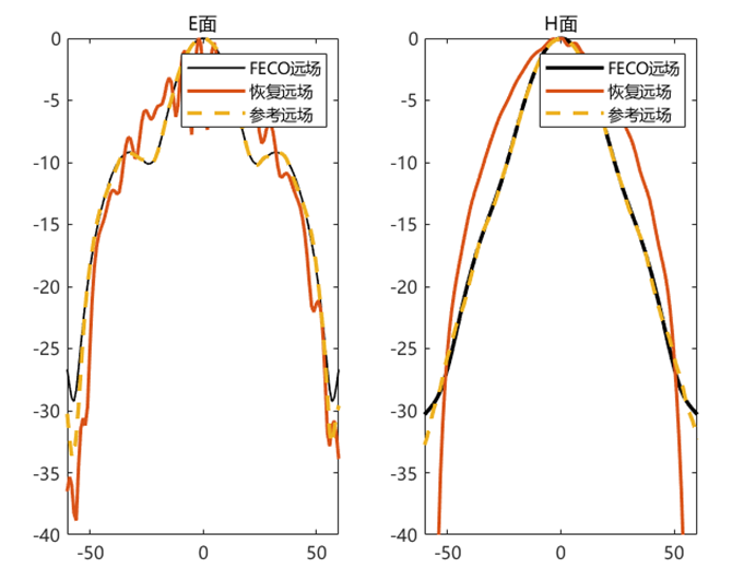
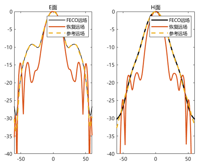
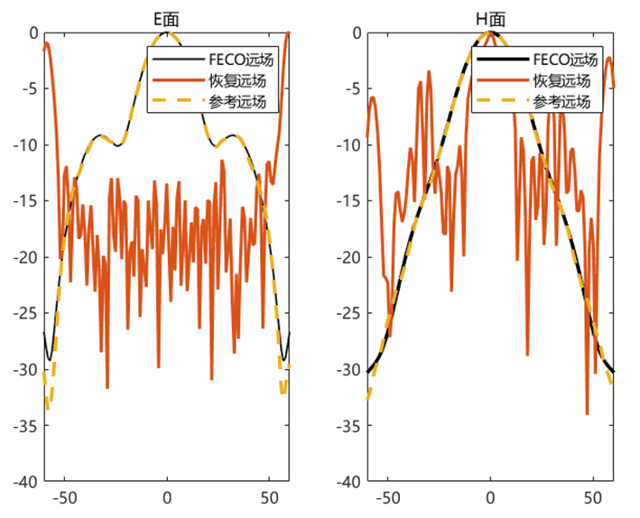
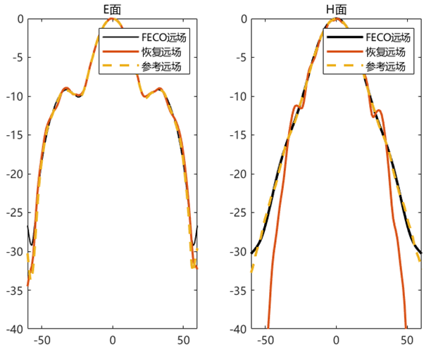
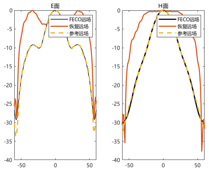
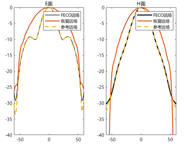
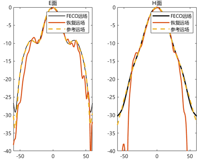
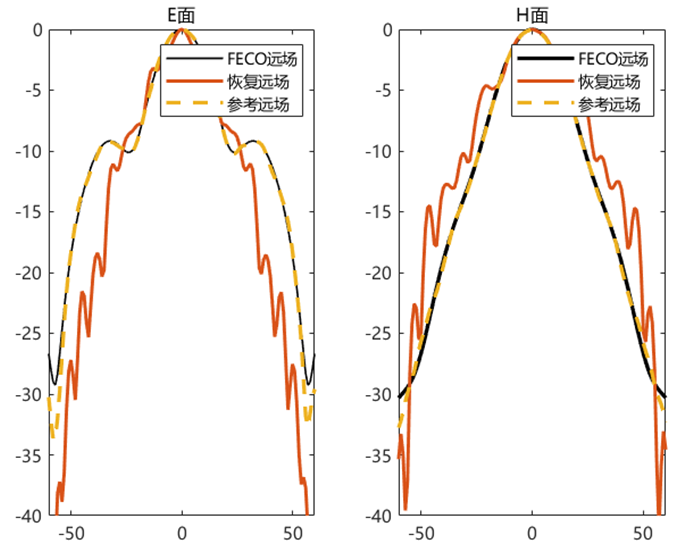
对比远场数据 为验证 PhaseRetrival 工具包的计算结果,使用其计算出的远场方向图与FECO导出的远场进行对比。
1 2 3 4 5 6 7 8 9 10 11 12 13 14 15 16 17 18 19 [EPLANE, HPLANE, Etot] = computerFF(theta, phi, Ex2, E2, k0, M, N, dx); [EPLANE2, HPLANE2, Etot2] = computerFF(theta, phi, Ex2, Ey2, k0, M, N, dx); Etot_Size = size (Etot); ffH_err = 20 * log10 (abs ((Etot(1 , :) - Etot2(1 , :)) / max (Etot2(1 , :)))); ffE_err = 20 * log10 (abs ((Etot(floor (Etot_Size(2 ) / 2 ), :)) - Etot2(floor (Etot_Size(2 ) / 2 ), :)) ./ max (Etot2(floor (Etot_Size(2 ) / 2 ), :))); ENL_H = 20 * log10 (mean (abs ((Etot(1 , :) - Etot2(1 , :)) / max (Etot2(1 , :))))); ENL_E = 20 * log10 (mean (abs ((Etot(floor (Etot_Size(2 ) / 2 ), :)) - Etot2(floor (Etot_Size(2 ) / 2 ), :)) ./ max (Etot2(floor (Etot_Size(2 ) / 2 ), :)))); ENL = 20 * log10 (mean (abs ((Etot - Etot2) / max (max (Etot2))), "all" )); far_data = importdata("E:\组会\其他\实验室历史文件\code\phase retrival\NFdata\ffdata.dat" ); xn1 = far_data.data(:, 1 ); yn1 = far_data.data(:, 2 ); yn2 = far_data.data(:, 3 );
辅助函数 下面是 PhaseRetrival 工具包在计算两个面衍射的时候,使用的辅助函数A 和 A的逆函数At。
1 2 3 4 5 6 7 8 9 10 11 12 13 14 15 16 17 18 19 20 21 22 23 24 25 26 27 28 29 30 31 32 33 34 35 36 function measurements = A (pixels) global numrows numcols num_fourier_masks masks padding dx; dk_X = 2 * pi / (numrows * dx); im = reshape (pixels, [numrows, numcols]); measurements = zeros (numrows / padding, numcols / padding, num_fourier_masks); for m = 1 :num_fourier_masks this_mask = squeeze (masks(:, :, m)); measurements_Padded = (fft2(ifftshift(im .* this_mask))) * dk_X * dk_X / (4 * pi * pi ); measurements(:, :, m) = measurements_Padded(1 :numrows / padding, 1 :numcols / padding); end measurements = measurements(:); end function pixels = At (measurements) global numrows numcols num_fourier_masks masks padding dx; dk_X = 2 * pi / (numrows * dx); im_reconstructed = zeros (numrows, numcols); measurements = reshape (measurements, [numrows / padding, numcols / padding, num_fourier_masks]); for m = 1 :num_fourier_masks this_mask = squeeze (masks(:, :, m)); this_measurements = squeeze (measurements(:, :, m)); im_reconstructed = im_reconstructed + conj (this_mask) .* fftshift(ifft2(this_measurements, numrows, numcols)) * numrows * numcols * dk_X * dk_X / (4 * pi * pi ); end pixels = im_reconstructed(:); end
使用U-Net 网络直接进行相位恢复 下面是最初直接使用tensorflow 搭建 U-Net 网络进行相位恢复的代码
数据读取 1 2 3 4 5 6 7 8 9 10 11 12 13 14 15 16 17 18 19 20 21 22 23 24 25 26 27 28 29 30 31 32 33 34 35 36 37 38 39 40 41 42 43 44 45 46 47 48 49 50 51 52 53 54 55 56 57 class PlaneData : def __init__ (self, file_name ): abs_temp = [] E_temp = [] phase_temp = [] f = open (file_name) E = f.read() if file_name.split('.' )[-1 ] == 'txt' : E = E.split('\n' )[2 :-1 ] elif file_name.split('.' )[-1 ] == 'efe' : E = E.split('\n' )[16 :-2 ] x = int (np.sqrt(len (E))) y = int (np.sqrt(len (E))) index_dot = file_name.find('-' ) distance_plane = int (file_name[index_dot - 1 ]) + float (file_name[index_dot + 1 ]) * 0.1 main_direction = 'y' for k in E: E_xp, E_yp, E_zp, E_xr, E_xi, E_yr, E_yi, E_zr, E_zi = k.split() E_x = complex (float (E_xr), float (E_xi)) E_y = complex (float (E_yr), float (E_yi)) E_z = complex (float (E_zr), float (E_zi)) if main_direction == 'y' : abs_temp.append(np.abs (E_y)) E_temp.append(E_y) phase = np.angle(E_y) phase_temp.append(phase) elif main_direction == 'x' : abs_temp.append(np.abs (E_x)) E_temp.append(E_x) phase = np.angle(E_x) phase_temp.append(phase) elif main_direction == 'z' : abs_temp.append(np.abs (E_z)) E_temp.append(E_z) phase = np.angle(E_z) phase_temp.append(phase) abs_pro = np.array(abs_temp).reshape((x, y)) E_temp = np.array(E_temp).reshape((x, y)) phase_pro = np.array(phase_temp).reshape((x, y)) self.abs = abs_pro[0 :96 , 0 :96 ] / np.max (abs_pro[0 :96 , 0 :96 ]) self.phase = phase_pro[0 :96 , 0 :96 ] self.E = E_temp[0 :96 , 0 :96 ] / np.max (np.abs (E_temp[0 :96 , 0 :96 ])) self.N = x - 1 self.distance = distance_plane plane_1 = PlaneData(r'DATA\l_6lamb_n_97_2-5lamb.efe' ) plane_2 = PlaneData(r'DATA\l_6lamb_n_97_3-0lamb.efe' ) plane_3 = PlaneData(r'DATA\l_6lamb_n_97_3-2lamb.efe' )
定义变量 1 2 3 4 5 6 7 8 9 10 11 12 13 14 15 16 17 18 dim = plane_1.N jqx = 0 jqy = 0 plane_W = dim plane_H = dim batch_size = 1 lamb = 299792458 / 1.65e9 pixelsize = lamb / 8 N = dim L = N * pixelsize Steps = 5000 LR = 0.01 noise_level = 0
定义网络结构 1 2 3 4 5 6 7 8 9 10 11 with tf.compat.v1.variable_scope('input' ): rand = tf.placeholder(shape=(dim, dim), dtype=tf.float32, name='noise' ) true_measure = tf.constant(plane_2.abs , dtype=tf.float32, name='diffraction' ) inpt = true_measure + rand with tf.compat.v1.variable_scope('inference' ): out = model_Unet.inference(inpt, plane_H, plane_W, batch_size) out = tf.reshape(out, [plane_H, plane_W])
引入物理衍射 1 2 3 out_calculate = Calculate_step.Phy(out, lamb, L, (plane_2.distance - plane_1.distance) * lamb, plane_1.abs , jqx, jqy, plane_H, plane_W)
上面 Calculate_step.Phy 函数用来模拟物理传播过程,与之前使用 PhaseRetrival 工具包进行相位恢复时的物理传播过程保持一致。
1 2 3 4 5 6 7 8 9 10 11 12 13 14 15 16 17 18 19 20 21 22 23 24 25 26 27 28 29 30 31 32 33 34 35 36 37 38 39 40 41 42 43 44 45 46 47 48 49 50 51 52 53 54 55 56 57 58 59 60 61 62 63 64 65 66 def Phy (fai_1, lamb, L, Z, E_1_abs, jqx, jqy, plane_H, plane_W ): M = int (fai_1.shape[1 ]) E_abs_1 = E_1_abs E_abs_1 = E_abs_1[jqx:jqx + plane_H, jqy:jqy + plane_W] E_abs_1 = E_abs_1 / np.max (E_abs_1) fai_1 = tf.cast(fai_1, dtype=tf.complex128) fai_1 = 1j * fai_1 U_in0 = tf.exp(fai_1) U_in = tf.multiply(U_in0, E_abs_1) U_in_fft = Myfftshift.fftshift(tf.signal.fft2d(U_in)) U_in_fft = tf.cast(U_in_fft, dtype=tf.complex128) fx = 1 / L x = np.linspace(-M / 2 , M / 2 - 1 , M) fx = (fx * x) [Fx, Fy] = np.meshgrid(fx, fx) k = 2 * math.pi / lamb Ax = 548 Ay = 426 Lx = L * 1000 Ly = L * 1000 Reliable_rate = 1 thea_x = Reliable_rate * np.arctan(((Lx - Ax) / 2 / 2.5 / lamb / 1000 )) thea_y = Reliable_rate * np.arctan(((Ly - Ay) / 2 / 2.5 / lamb / 1000 )) G1 = (1 - lamb * lamb * (Fx * Fx / np.sin(thea_x) / np.sin(thea_x) + Fy * Fy)) G2 = (1 - lamb * lamb * (Fx * Fx + Fy * Fy / np.sin(thea_y) / np.sin(thea_y))) G = (1 - lamb * lamb * (Fx * Fx + Fy * Fy)) H = np.ones_like(G) * 1j for i in range (H.shape[0 ]): for j in range (H.shape[1 ]): if G[i, j] >= 0 : temp = k * (-1 * Z) * np.sqrt(G[i, j]) H[i, j] = np.exp(1j * temp) else : temp = k * (1j * Z) * np.sqrt(1j * G[i, j] * 1j ) H[i, j] = np.exp(-1 * temp) H = tf.cast(H, dtype=tf.complex128) U_out_fft = tf.multiply(U_in_fft, H) U_out = tf.signal.ifft2d(Myfftshift.ifftshift(U_out_fft)) U_out_abs = tf.abs (U_out) temp = tf.reduce_max(tf.reduce_max(U_out_abs)) U_out = tf.abs (U_out) / temp return U_out
神经网络补充 1 2 3 4 5 6 loss_m = tf.compat.v1.losses.mean_squared_error(out_calculate, true_measure) optimizer = tf.compat.v1.train.AdamOptimizer(learning_rate=LR) update_ops = tf.compat.v1.get_collection(tf.compat.v1.GraphKeys.UPDATE_OPS)
神经网络初始化 1 2 3 4 5 6 7 8 9 10 11 12 13 with tf.control_dependencies(update_ops): train_op = optimizer.minimize(loss_m) saver = tf.compat.v1.train.Saver() with tf.compat.v1.Session() as sess: sess.run(tf.global_variables_initializer()) m_loss = np.zeros([Steps, 1 ]) temp_m_loss = []
网络迭代优化 1 2 3 4 5 6 7 8 9 10 11 12 13 14 15 for step in range (Steps): new_rand = np.random.uniform(0 , noise_level, size=(dim, dim)) sess.run([train_op], feed_dict={rand: new_rand}) loss_measure = sess.run(loss_m, feed_dict={rand: new_rand}) m_loss[step] = loss_measure print ('Step:%d Measure loss:%f' % (step, loss_measure)) new_rand = np.random.uniform(0 , 0.0 , size=(dim, dim)) pha_out = sess.run(out, feed_dict={rand: new_rand}).reshape(dim, dim) out_calculate_temp = sess.run(out_calculate, feed_dict={rand: new_rand}).reshape(dim, dim)
使用U-Net 网络源重构进行相位恢复 下面是通过源重构进行相位恢复,把上面物理衍射的物理过程改为格林公式,模拟等效源在空间中的辐射过程。
模型差异 其机器学习相关的大量代码——网络结构、初始化、迭代过程——与上一个保持一致,只是物理过程部分的代码不同,下面只展示不同部分。
1 2 3 4 5 6 7 8 9 sample1_cords = Calculate_step.set_cords(-1 * int (N / 2 ) * dx, int (N / 2 ) * dy, dx, dy, plane_RS.distance * lamda) source_cords = Calculate_step.set_cords(-1 * int (N / 2 ) * dx, int (N / 2 ) * dy, dx, dy, plane_RS.distance * lamda * 0.8 ) g = Calculate_step.green_function(source_cords, sample1_cords, k, dx, dy) out_calculate = tf.abs (g @ out) out_calculate = tf.reshape(out_calculate, [dim, dim])
1 2 3 4 5 6 7 8 9 10 11 12 13 def set_cords (begin, end, dx, dy, Z ): x_d = np.arange(begin, end, dx) y_d = np.arange(begin, end, dy) [x_grid, y_grid] = np.meshgrid(x_d, y_d) z_grid = Z * np.ones_like(x_grid) x_cords = x_grid.reshape(-1 , 1 ) y_cords = y_grid.reshape(-1 , 1 ) z_cords = z_grid.reshape(-1 , 1 ) return_cords = np.hstack((y_cords, x_cords, z_cords)) return return_cords
1 2 3 4 5 6 7 8 9 10 11 12 13 14 15 16 17 18 def green_function (source_xy, sample_xy, k, dx, dy ): x_source = source_xy[:, 0 ] y_source = source_xy[:, 1 ] z_source = source_xy[:, 2 ] x_sample = sample_xy[:, 0 ] y_sample = sample_xy[:, 1 ] z_sample = sample_xy[:, 2 ] g = np.zeros((len (x_sample), len (x_source)), dtype=complex ) for m in range (len (x_sample)): R_ij = np.sqrt((x_sample[m] - x_source) ** 2 + (y_sample[m] - y_source) ** 2 + (z_sample[m] - z_source) ** 2 ) g[m, :] = 1 / (4 * np.pi) * (np.exp(-1j * k * R_ij) / R_ij ** 2 ) * ((z_sample[m] - z_source) * (1j * k + 1 / R_ij)) * dx * dy return g
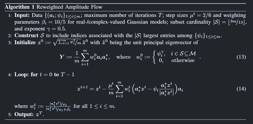
使用全连接神经网络进行相位恢复 论文复现 首先,下面是对 PhaseRetrival 工具包中相位恢复相关论文中提到的原理复现。这一部分并不涉及机器学习,是传统的相位恢复算法——使用加权最大相关初始化,并用加权梯度流进行迭代。
按照给定的形状随机生成实数信号(y、A、x)
1 2 3 4 5 6 7 8 9 def generate_data (n, m ): x = np.random.randn(n) x = x / np.linalg.norm(x) A = np.random.randn(m, n) y = np.abs (A @ x) return A, y, x
定义初始化方法
1 2 3 4 5 6 7 8 9 10 11 12 13 14 15 16 17 def weighted_max_correlation_init (A, y, S_size ): m, n = A.shape S = np.argsort(y)[-S_size:] A_S = A[S, :] y_S = y[S] gamma = 0.5 weights = y_S ** gamma Y = (A_S.T * weights) @ A_S / S_size _, _, Vt = svds(Y, k=1 ) z0 = Vt[0 ] norm_estimate = np.sqrt(np.mean(y ** 2 )) z0 = z0 * norm_estimate return z0
定义优化方法——加权幅流法
1 2 3 4 5 6 7 8 9 10 11 12 13 14 15 16 17 18 def reweighted_amplitude_flow (A, y, z0, max_iter=3000 , mu=0.5 , beta=5 ): m, n = A.shape z = z0.copy() for t in range (max_iter): Az = A @ z Az_abs = np.abs (Az) ratios = Az_abs / y weights = 1 / (1 + beta / ratios) gradient = (A.T @ (weights * (Az - y * (Az / Az_abs)))) / m z = z - mu * gradient if np.linalg.norm(gradient) < 1e-6 : break return z
主函数
1 2 3 4 5 6 7 8 9 10 11 12 13 14 15 16 def main (): n = 1000 m = 2 * n - 1 S_size = int (3 * m / 13 ) A, y, x = generate_data(n, m) z0 = weighted_max_correlation_init(A, y, S_size) z_hat = reweighted_amplitude_flow(A, y, z0) error = np.linalg.norm(z_hat - x) / np.linalg.norm(x) print (f"Recovery error: {error} " )
引入神经网络实现 下面把神经网络引入,根据之前同学提醒,打算使用端对端的神经网络,通过输入A与y,直接得到待求的x。
1 2 3 4 5 6 def generate_data (n, m ): x = np.random.randn(n) A = np.random.randn(m, n) y = np.abs (A @ x) return A, y, x
1 2 3 4 5 6 7 8 9 10 11 12 13 14 15 16 17 18 19 20 21 22 class SignalRecoveryModel (nn.Module): def __init__ (self, m, n ): super (SignalRecoveryModel, self).__init__() self.input_size = m * n + m self.fc1 = nn.Linear(self.input_size, 512 ) self.fc2 = nn.Linear(512 , 256 ) self.fc3 = nn.Linear(256 , n) self.relu = nn.ReLU() def forward (self, A, y ): A_flat = A.view(-1 ) y_flat = y.view(-1 ) x_input = torch.cat((A_flat, y_flat), dim=0 ) x_input = x_input.unsqueeze(0 ) x = self.relu(self.fc1(x_input)) x = self.relu(self.fc2(x)) x = self.fc3(x) return x.squeeze(0 )
1 2 3 4 5 6 7 8 9 10 11 12 13 14 15 16 17 18 19 20 21 22 23 24 25 26 27 28 29 30 31 32 33 34 35 36 37 38 def main (): n = 97 * 2 m = 2 * n A, y, x = generate_data(n, m) A_tensor = torch.FloatTensor(A) y_tensor = torch.FloatTensor(y) x_tensor = torch.FloatTensor(x) model = SignalRecoveryModel(m, n) criterion = nn.MSELoss() optimizer = optim.Adam(model.parameters(), lr=0.001 ) num_epochs = 1000 for epoch in range (num_epochs): model.train() optimizer.zero_grad() outputs = model(A_tensor, y_tensor) loss = criterion(outputs, x_tensor) loss.backward() optimizer.step() if (epoch + 1 ) % 100 == 0 : print (f'Epoch [{epoch + 1 } /{num_epochs} ], Loss: {loss.item():.4 f} ' ) model.eval () with torch.no_grad(): z_hat = model(A_tensor, y_tensor).numpy() error = np.linalg.norm(z_hat - x) / np.linalg.norm(x) print (f"Recovery error: {error} " )
复数改进 上面的代码只针对实数的情况,但在相位恢复中的数据都是复数,目前的神经网络只支持实数,所以需要对其进行改进,以满足复数的需要,下面是改进后的代码。
1 2 3 4 5 6 7 8 9 10 11 12 13 def generate_data (n, m ): x = np.random.randn(n) + 1j * np.random.randn(n) x = x / np.linalg.norm(x) A = np.random.randn(m, n) + 1j * np.random.randn(m, n) y = np.abs (A @ x) return A, y, x
1 2 3 4 5 6 7 8 9 10 11 12 13 14 15 16 17 18 19 20 21 22 23 24 25 26 27 28 29 30 class ComplexSignalRecoveryModel (nn.Module): def __init__ (self, m, n ): super (ComplexSignalRecoveryModel, self).__init__() self.input_size = 2 * m * n + m self.output_size = 2 * n self.fc1 = nn.Linear(self.input_size, 2048 ) self.fc2 = nn.Linear(2048 , 1024 ) self.fc3 = nn.Linear(1024 , self.output_size) self.relu = nn.ReLU() def forward (self, A_real_flat, A_imag_flat, y_flat ): x_input = torch.cat([A_real_flat, A_imag_flat, y_flat], dim=0 ) x_input = x_input.unsqueeze(0 ) x = self.relu(self.fc1(x_input)) x = self.relu(self.fc2(x)) x = self.fc3(x) x_out = x.squeeze(0 ) x_real = x_out[:self.output_size // 2 ] x_imag = x_out[self.output_size // 2 :] return x_real, x_imag
1 2 3 4 5 6 7 8 9 10 11 12 13 14 15 16 17 18 19 20 21 22 23 24 25 26 27 28 29 30 31 32 33 34 35 36 37 38 39 40 41 42 43 44 45 46 47 48 49 50 51 52 53 def main (): n = 25 m = 2 * n - 1 A, y, x = generate_data(n, m) x_real_true = np.real(x) x_imag_true = np.imag(x) A_real = np.real(A).flatten() A_imag = np.imag(A).flatten() y_flat = y.flatten() A_real_tensor = torch.FloatTensor(A_real) A_imag_tensor = torch.FloatTensor(A_imag) y_tensor = torch.FloatTensor(y_flat) x_real_tensor = torch.FloatTensor(x_real_true) x_imag_tensor = torch.FloatTensor(x_imag_true) model = ComplexSignalRecoveryModel(m, n) criterion = nn.MSELoss() optimizer = optim.Adam(model.parameters(), lr=0.001 ) num_epochs = 1000 for epoch in range (num_epochs): model.train() optimizer.zero_grad() x_real_pred, x_imag_pred = model(A_real_tensor, A_imag_tensor, y_tensor) loss_real = criterion(x_real_pred, x_real_tensor) loss_imag = criterion(x_imag_pred, x_imag_tensor) total_loss = loss_real + loss_imag total_loss.backward() optimizer.step() if (epoch + 1 ) % 100 == 0 : print (f'Epoch [{epoch + 1 } /{num_epochs} ], Loss: {total_loss.item():.4 f} ' ) model.eval () with torch.no_grad(): x_real_pred, x_imag_pred = model(A_real_tensor, A_imag_tensor, y_tensor) z_hat = x_real_pred.numpy() + 1j * x_imag_pred.numpy() error = np.linalg.norm(z_hat - x) / np.linalg.norm(x) print (f"Recovery error: {error} " )
验证传播函数的正确性 这一部分用来验证传播函数部分代码的正确性,共有两个部分。第一部分是与之前 PhaseRetrival 工具包一样,验证衍射过程的正确性;第二部分是因为在神经网络中需要测量矩阵A的显示表达,所以还需验证其正确性。
首先是衍射过程中函数A和A的逆函数At的实现:
1 2 3 4 5 6 7 8 9 10 11 12 13 def A_function (pixels, masks, padding, dx ): numrows, numcols = masks.shape[:2 ] im = pixels.reshape(numrows, numcols) measurements = np.zeros((numrows // padding, numcols // padding, masks.shape[2 ]), dtype=np.complex128) dk_X = 2 * np.pi / (numrows * dx) for m in range (masks.shape[2 ]): masked = im * masks[:, :, m] ft = np.fft.fft2(np.fft.ifftshift(masked)) measurements[:, :, m] = ft[:numrows // padding, :numcols // padding] * (dk_X ** 2 ) / (4 * np.pi ** 2 ) return measurements.ravel(order='F' )
1 2 3 4 5 6 7 8 9 10 11 12 13 14 def At_function (measurements, numrows, numcols, num_fourier_masks, masks, padding, dx ): dk_X = 2 * np.pi / (numrows * dx) im_reconstructed = np.zeros((numrows, numcols), dtype=complex ) measurements = np.reshape(measurements, (numrows // padding, numcols // padding, num_fourier_masks), order='F' ) for m in range (num_fourier_masks): this_mask = np.squeeze(masks[:, :, m]) this_measurements = np.squeeze(measurements[:, :, m]) im_reconstructed += np.conj(this_mask) * np.fft.fftshift(np.fft.ifft2(this_measurements, s=(numrows, numcols))) * numrows * numcols * dk_X * dk_X / (4 * np.pi * np.pi) pixels = im_reconstructed.ravel(order='F' ) return pixels
下面是测量矩阵A的显示表达函数:
1 2 3 4 5 6 7 8 9 10 11 12 13 def At_function (measurements, numrows, numcols, num_fourier_masks, masks, padding, dx ): dk_X = 2 * np.pi / (numrows * dx) im_reconstructed = np.zeros((numrows, numcols), dtype=complex ) measurements = np.reshape(measurements, (numrows // padding, numcols // padding, num_fourier_masks), order='F' ) for m in range (num_fourier_masks): this_mask = np.squeeze(masks[:, :, m]) this_measurements = np.squeeze(measurements[:, :, m]) im_reconstructed += np.conj(this_mask) * np.fft.fftshift(np.fft.ifft2(this_measurements, s=(numrows, numcols))) * numrows * numcols * dk_X * dk_X / (4 * np.pi * np.pi) pixels = im_reconstructed.ravel(order='F' ) return pixels
功能整合 整合上面提到的功能,在下面的代码中,可以完成三个主要的功能:
1 process = ['train' , 'test' , 'trained_test' ]
'train':使用随机生成的数据训练模型'test':不使用神经网络的部分,仅仅验证传播函数的正确性'trained_test':对训练好的模型进行测试,目前是使用重新随机生成的数据进行测试,接下来还会补充使用FECO导出的电场数据进行测试
1 2 3 4 5 6 7 8 9 10 11 12 13 14 15 16 17 18 19 20 21 22 23 24 25 26 27 28 29 30 31 32 33 34 35 36 37 38 39 40 41 42 43 44 45 46 47 48 49 50 51 52 53 54 55 56 57 58 59 60 61 62 63 64 65 66 67 68 69 if 'train' in process: device = torch.device('cuda' if (torch.cuda.is_available() and FLAG_GPU) else 'cpu' ) A, y, x = generate_data(n, m) file_path = r"E:\PhysenNet_inversion\DATA\process_DATA\test_A.npy" np.save(file_path, A) print ("已创建并保存test_A.npy数据" ) model = ComplexSignalRecoveryModel(m, n).to(device) criterion = nn.MSELoss() optimizer = optim.Adam(model.parameters(), lr=0.001 ) num_epochs = 1000 for epoch in range (num_epochs): model.train() optimizer.zero_grad() A, y, x = generate_data(n, m, A) x_real_true = np.real(x) x_imag_true = np.imag(x) A_real = np.real(A).ravel(order='F' ) A_imag = np.imag(A).ravel(order='F' ) y_flat = y.flatten() A_real_tensor = torch.FloatTensor(A_real).to(device) A_imag_tensor = torch.FloatTensor(A_imag).to(device) y_tensor = torch.FloatTensor(y_flat).to(device) x_real_tensor = torch.FloatTensor(x_real_true).to(device) x_imag_tensor = torch.FloatTensor(x_imag_true).to(device) x_real_pred, x_imag_pred = model(A_real_tensor, A_imag_tensor, y_tensor) loss_real = criterion(x_real_pred, x_real_tensor) loss_imag = criterion(x_imag_pred, x_imag_tensor) total_loss = loss_real + loss_imag total_loss.backward() optimizer.step() if (epoch + 1 ) % 100 == 0 : print (f'Epoch [{epoch + 1 } /{num_epochs} ], Loss: {total_loss.item():.4 f} ' ) model.eval () with torch.no_grad(): x_real_pred, x_imag_pred = model(A_real_tensor, A_imag_tensor, y_tensor) z_hat = x_real_pred.cpu().numpy() + 1j * x_imag_pred.cpu().numpy() error = np.linalg.norm(z_hat - x) / np.linalg.norm(x) error = mean_squared_error(np.real(z_hat), np.real(x)) + mean_squared_error(np.imag(z_hat), np.imag(x)) print (f"Recovery error: {error} " ) model_path = r"E:\PhysenNet_inversion\DATA\process_DATA\complex_signal_model.pth" torch.save(model, model_path) print (f"模型已保存到 {model_path} " )
1 2 3 4 5 6 7 8 9 10 11 12 13 14 15 16 17 18 19 20 21 22 23 24 25 26 27 28 29 30 31 32 33 34 35 36 37 38 39 40 41 42 43 44 45 46 47 48 49 50 51 52 53 54 55 56 57 58 59 60 61 62 63 64 65 66 67 68 69 70 71 72 73 74 75 76 77 78 79 80 81 82 83 84 85 86 87 88 89 90 91 92 93 94 95 96 97 98 99 100 101 102 103 104 105 106 107 108 109 110 111 112 113 114 115 116 117 118 119 120 121 122 123 124 125 126 127 128 129 130 131 132 133 134 135 136 137 138 139 140 141 142 143 144 145 146 147 148 149 150 151 152 153 154 155 156 157 158 159 160 161 if 'test' in process: f = 1.65e9 lamda = constants.speed_of_light / f k0 = 2 * np.pi / lamda dtheta = np.pi / 180 dphi = np.pi / 180 theta = np.arange(-np.pi / 2 , np.pi / 2 + dtheta, dtheta) phi = np.arange(0 , np.pi + dphi, dphi) NF_data1 = r'E:\组会\其他\实验室历史文件\code\phase retrival\NFdata\NearField3_10X10P25_0P25.efe' NF_data2 = r'E:\组会\其他\实验室历史文件\code\phase retrival\NFdata\NearField4_10X10P25_0P25.efe' NF_data3 = r'E:\组会\其他\实验室历史文件\code\phase retrival\NFdata\NearField5_10X10P25_0P25.efe' dz_values = [0 , 1 ] z0, z1, z2 = 3.0 * lamda, 4.0 * lamda, 5.0 * lamda Reliable_rate = 1 Ex1, Ey1, xd1, yd1, z = load_NF(NF_data1) Ex2, Ey2, xd2, yd2, z = load_NF(NF_data2) Ex3, Ey3, xd3, yd3, z = load_NF(NF_data3) Ey1_1D = Ey1.flatten(order='F' ) Ey2_1D = Ey2.flatten(order='F' ) Ey3_1D = Ey3.flatten(order='F' ) M = int (len (xd2)) N = int (len (yd2)) dx = float (xd2[1 ] - xd2[0 ]) dy = float (yd2[1 ] - yd2[0 ]) padding = 1 MI = padding * M NI = padding * N m = np.arange(-MI // 2 , MI // 2 ) n = np.arange(-NI // 2 , NI // 2 ) k_X_Rectangular = 2 * np.pi * m / (MI * dx) k_Y_Rectangular = 2 * np.pi * n / (NI * dy) dk_X = k_X_Rectangular[1 ] - k_X_Rectangular[0 ] dk_Y = k_Y_Rectangular[1 ] - k_Y_Rectangular[0 ] k_Y_Rectangular_Grid, k_X_Rectangular_Grid = np.meshgrid(k_Y_Rectangular, k_X_Rectangular) kz = np.sqrt(k0 ** 2 - k_X_Rectangular_Grid ** 2 - k_Y_Rectangular_Grid ** 2 + 0j ) W = 0.55 H = 0.428 w = dx * (M - 1 ) h = dy * (N - 1 ) thetax_sure = Reliable_rate * np.arctan(0.5 * (w - W) / z1) thetay_sure = Reliable_rate * np.arctan(0.5 * (h - H) / z1) file_path = r"E:\PhysenNet_inversion\DATA\process_DATA\UR.npy" if os.path.isfile(file_path): print ("UR.npy 文件存在" ) UR = np.load(file_path) print ("成功加载 UR.npy 文件" ) else : print ("UR.npy 文件不存在" ) UR = np.zeros((MI, NI), dtype=int ) for i in range (MI): for j in range (NI): condition1 = (k_X_Rectangular[i] ** 2 / (k0 * np.sin(thetax_sure)) ** 2 + k_Y_Rectangular[j] ** 2 / k0 ** 2 ) < 1.0 condition2 = (k_X_Rectangular[i] ** 2 / k0 ** 2 + k_Y_Rectangular[j] ** 2 / (k0 * np.sin(thetay_sure)) ** 2 ) < 1.0 if condition1 and condition2: UR[i, j] = 1 np.save(file_path, UR) print ("已创建并保存UR.npy数据" ) fy1 = np.fft.fftshift(np.fft.ifft2(Ey2, s=(MI, NI))) * MI * NI * dx * dy fy_Magnitude = 20 * np.log10(np.abs (fy1)) fy_H_Magnitude = 20 * np.log10(np.abs (fy1 * UR)) numrows, numcols = k_Y_Rectangular_Grid.shape num_fourier_masks = 2 isim = np.imag(kz) != 0 kz[isim] = -1 * kz[isim] file_path = r"E:\PhysenNet_inversion\DATA\process_DATA\masks.npy" if os.path.isfile(file_path): print ("masks.npy 文件存在" ) masks = np.load(file_path) print ("成功加载 masks.npy 文件" ) else : print ("masks.npy 文件不存在" ) masks = np.zeros((numrows, numcols, num_fourier_masks), dtype=np.complex128) for i in range (num_fourier_masks): phase = -1j * kz * dz_values[i] * lamda masks[:, :, i] = UR * np.exp(phase) np.save(file_path, masks) print ("已创建并保存masks.npy数据" ) fy2 = np.fft.fftshift(np.fft.ifft2(Ey2, s=(MI, NI))) * MI * NI * dx * dy x = fy2.flatten() file_path = r"E:\PhysenNet_inversion\DATA\process_DATA\A.npy" if os.path.isfile(file_path): print ("A.npy 文件存在" ) A = np.load(file_path) print ("成功加载 A.npy 文件" ) else : print ("A.npy 文件不存在" ) A = construct_A_matrix(masks, padding, dx) np.save(file_path, A) print ("已创建并保存A.npy数据" ) b_cal = np.abs (A @ x) b_real = np.concatenate([np.abs (Ey2_1D.ravel(order='F' )), np.abs (Ey3_1D.ravel(order='F' ))]) b_err_1 = np.sqrt(np.sum ((np.abs (b_real) - b_cal) ** 2 ) / np.sum (b_cal ** 2 )) b_err_2 = np.abs ((b_real - b_cal) / b_cal) b_err = b_err_2.reshape((numrows // padding, numcols // padding, num_fourier_masks)) E1_err = np.squeeze(b_err[:, :, 0 ]) E2_err = np.squeeze(b_err[:, :, 1 ])
1 2 3 4 5 6 7 8 9 10 11 12 13 14 15 16 17 18 19 20 21 22 23 24 25 26 27 28 29 30 31 32 33 34 35 36 37 38 39 40 41 42 if 'trained_test' in process: device = torch.device('cuda' if (torch.cuda.is_available() and FLAG_GPU) else 'cpu' ) model_path = r"E:\PhysenNet_inversion\DATA\process_DATA\complex_signal_model.pth" if os.path.exists(model_path): print ("发现训练模型,加载模型中..." ) model = torch.load(model_path).to(device) A, y, x = generate_data(n, m) file_path = r"E:\PhysenNet_inversion\DATA\process_DATA\test_A.npy" if os.path.isfile(file_path): print ("test_A.npy 文件存在" ) A = np.load(file_path) print ("成功加载 test_A.npy 文件" ) else : pass A_real = np.real(A).ravel(order='F' ) A_imag = np.imag(A).ravel(order='F' ) y_flat = y.flatten() A_real_tensor = torch.FloatTensor(A_real).to(device) A_imag_tensor = torch.FloatTensor(A_imag).to(device) y_tensor = torch.FloatTensor(y_flat).to(device) model.eval () with torch.no_grad(): x_real_pred, x_imag_pred = model(A_real_tensor, A_imag_tensor, y_tensor) z_hat = x_real_pred.cpu().numpy() + 1j * x_imag_pred.cpu().numpy() error = np.linalg.norm(z_hat - x) / np.linalg.norm(x) error = mean_squared_error(np.real(z_hat), np.real(x)) + mean_squared_error(np.imag(z_hat), np.imag(x)) print (f"Recovery error: {error} " )
使用 initWeighted 初始化 使用 Python 对 PhaseRetrival 工具包进行改写,并验证改写代码的正确性,验证思路如下:
使用相同的初始数据,得到初始化的结果,与 PhaseRetrival 工具包计算得到的结果进行对比
把Python计算得到的结果带入到 PhaseRetrival 工具包,使用相同的迭代方法,看是否可以收敛到真实解
代码部分 1 2 3 4 5 6 7 8 9 10 11 12 13 14 15 16 17 18 19 20 21 22 23 24 25 26 27 28 29 30 31 32 33 34 35 36 37 38 39 40 41 42 43 44 45 46 47 48 49 50 51 52 53 54 55 56 57 58 59 60 61 62 63 64 65 66 67 68 69 70 71 72 73 74 75 76 77 78 79 80 81 82 83 84 85 86 87 88 89 90 91 92 93 94 95 96 97 98 99 100 101 102 103 104 105 106 107 108 109 110 111 112 113 114 115 116 117 118 119 120 121 122 123 124 125 126 127 128 129 130 131 132 133 134 135 136 137 138 139 140 141 142 143 144 145 146 147 148 149 150 151 152 153 154 155 156 157 158 159 160 161 162 163 164 165 166 167 168 169 170 171 172 173 174 175 176 177 178 179 180 181 182 183 184 185 186 187 188 189 190 191 192 193 194 195 196 197 198 199 200 201 202 203 204 205 206 207 208 209 210 211 212 213 214 215 216 217 218 219 220 221 222 223 224 225 226 227 228 229 230 231 232 233 234 235 236 237 238 239 240 241 242 243 244 245 246 247 248 249 250 251 252 253 254 255 256 257 258 259 260 261 262 263 264 265 266 267 268 269 270 271 272 273 274 275 276 277 278 279 280 281 282 283 284 285 286 287 288 289 290 291 292 293 294 295 296 297 298 299 300 301 302 303 304 305 306 307 308 309 310 311 312 313 314 315 316 317 318 319 320 321 322 323 324 325 326 327 328 329 330 331 332 333 334 335 336 337 338 import warningsimport matplotlib.pyplot as pltimport numpy as npfrom scipy.sparse.linalg import LinearOperator, eigsimport osfrom scipy import constantswarnings.filterwarnings("ignore" ) plt.rcParams['font.sans-serif' ] = ['SimHei' ] plt.rcParams['axes.unicode_minus' ] = False def load_NF (file_path ): near_Efield = np.loadtxt(file_path) xn = near_Efield[:, 0 ] yn = near_Efield[:, 1 ] zn = near_Efield[:, 2 ] z = zn[0 ] Ex = near_Efield[:, 3 ] + 1j * near_Efield[:, 4 ] Ey = near_Efield[:, 5 ] + 1j * near_Efield[:, 6 ] LM = np.where(yn == yn[0 ])[0 ] M = len (LM) N = len (xn) // M xd = np.linspace(xn.min (), xn.max (), M) yd = np.linspace(yn.min (), yn.max (), N) Ex_matrix = Ex.reshape(M, N).T Ey_matrix = Ey.reshape(M, N).T return Ex_matrix, Ey_matrix, xd, yd, z def setup_parameters (): """初始化所有物理参数和路径""" params = { 'f' : 1.65e9 , 'dz_values' : [0 , 1 ], 'z0' : 3.0 * constants.speed_of_light / 1.65e9 , 'Reliable_rate' : 0.8 , 'NF_paths' : [ r'E:\组会\其他\实验室历史文件\code\phase retrival\NFdata\NearField3_10X10P25_0P25.efe' , r'E:\组会\其他\实验室历史文件\code\phase retrival\NFdata\NearField4_10X10P25_0P25.efe' , r'E:\组会\其他\实验室历史文件\code\phase retrival\NFdata\NearField5_10X10P25_0P25.efe' ], 'UR_path' : r"E:\PhysenNet_inversion\DATA\process_DATA\UR.npy" , 'masks_path' : r"E:\PhysenNet_inversion\DATA\process_DATA\masks.npy" , 'padding' : 2 , 'num_fourier_masks' : 2 , 'W' : 0.55 , 'H' : 0.428 } lamda = constants.speed_of_light / params['f' ] params.update({ 'lamda' : lamda, 'k0' : 2 * np.pi / lamda, 'dtheta' : np.pi / 180 , 'dphi' : np.pi / 180 }) Ey_list = [] for path in params['NF_paths' ]: Ex_matrix, Ey_matrix, xd, yd, z = load_NF(path) Ey_list.append(Ey_matrix) params.update({ 'M' : len (xd), 'N' : len (yd), 'dx' : float (xd[1 ] - xd[0 ]), 'dy' : float (yd[1 ] - yd[0 ]) }) params.update({ 'MI' : params['M' ] * params['padding' ], 'NI' : params['N' ] * params['padding' ], 'Ey_data' : Ey_list }) m = np.arange(-params['MI' ] // 2 , params['MI' ] // 2 ) n = np.arange(-params['NI' ] // 2 , params['NI' ] // 2 ) k_X = 2 * np.pi * m / (params['MI' ] * params['dx' ]) k_Y = 2 * np.pi * n / (params['NI' ] * params['dy' ]) k_Y_grid, k_X_grid = np.meshgrid(k_Y, k_X) kz = np.sqrt(params['k0' ] ** 2 - k_X_grid ** 2 - k_Y_grid ** 2 + 0j ) kz[np.imag(kz) != 0 ] *= -1 if not os.path.exists(params['UR_path' ]): generate_UR_matrix(params, k_X, k_Y) UR = np.load(params['UR_path' ]) if not os.path.exists(params['masks_path' ]): generate_masks(params, UR, kz) masks = np.load(params['masks_path' ]) params.update({ 'masks' : masks }) return params def generate_UR_matrix (params, k_X, k_Y ): """生成可靠性区域矩阵""" print ("生成UR矩阵..." ) UR = np.zeros((params['MI' ], params['NI' ]), dtype=int ) w = params['dx' ] * (params['M' ] - 1 ) h = params['dy' ] * (params['N' ] - 1 ) thetax = params['Reliable_rate' ] * np.arctan(0.5 * (w - params['W' ]) / params['z0' ]) thetay = params['Reliable_rate' ] * np.arctan(0.5 * (h - params['H' ]) / params['z0' ]) for i in range (params['MI' ]): for j in range (params['NI' ]): condition1 = (k_X[i] ** 2 / (params['k0' ] * np.sin(thetax)) ** 2 + k_Y[j] ** 2 / params['k0' ] ** 2 ) < 1.0 condition2 = (k_X[i] ** 2 / params['k0' ] ** 2 + k_Y[j] ** 2 / (params['k0' ] * np.sin(thetay)) ** 2 ) < 1.0 if condition1 and condition2: UR[i, j] = 1 np.save(params['UR_path' ], UR) def generate_masks (params, UR, kz ): """生成傅里叶掩码""" print ("生成masks矩阵..." ) masks = np.zeros((params['MI' ], params['NI' ], params['num_fourier_masks' ]), dtype=np.complex128) for m in range (params['num_fourier_masks' ]): phase = -1j * kz * params['dz_values' ][m] * params['lamda' ] masks[:, :, m] = UR * np.exp(phase) np.save(params['masks_path' ], masks) def A_function (pixels, masks, padding, dx ): """A操作符:空间域 -> 截断傅里叶测量值""" numrows, numcols = masks.shape[:2 ] im = pixels.reshape(numrows, numcols) measurements = np.zeros((numrows // padding, numcols // padding, masks.shape[2 ]), dtype=np.complex128) dk_X = 2 * np.pi / (numrows * dx) scale = (dk_X ** 2 ) / (4 * np.pi ** 2 ) for m in range (masks.shape[2 ]): masked = im * masks[:, :, m] ft = np.fft.fft2(np.fft.ifftshift(masked)) measurements[:, :, m] = ft[:numrows // padding, :numcols // padding] * scale return measurements.ravel(order='F' ) def At_function (measurements, numrows, numcols, num_fourier_masks, masks, padding, dx ): """At操作符:测量值 -> 空间域重建""" dk_X = 2 * np.pi / (numrows * dx) scale = numrows * numcols * (dk_X ** 2 ) / (4 * np.pi ** 2 ) im_recon = np.zeros((numrows, numcols), dtype=complex ) measurements = measurements.reshape( (numrows // padding, numcols // padding, num_fourier_masks), order='F' ) for m in range (num_fourier_masks): meas_slice = measurements[:, :, m] full_ft = np.zeros((numrows, numcols), dtype=np.complex128) full_ft[:numrows // padding, :numcols // padding] = meas_slice recon = np.fft.fftshift(np.fft.ifft2(full_ft)) * scale im_recon += np.conj(masks[:, :, m]) * recon return im_recon.ravel(order='F' ) def validate_results (x2_true, x1_true, params ): b_cal = np.abs (A_function(x1_true, np.load(params['masks_path' ]), params['padding' ], params['dx' ])) b_real = np.concatenate([np.abs (params['Ey_data' ][1 ]).flatten(order='F' ), np.abs (params['Ey_data' ][2 ]).flatten(order='F' )]) err = np.sqrt(np.sum ((np.abs (b_real) - b_cal) ** 2 ) / np.sum (b_cal ** 2 )) print (f"物理衍射相对误差: {err:.4 e} " ) def initWeighted (A, At, b0, n, params, verbose=True ): """ 重加权振幅流(RAF)算法的加权初始化器 参数: A: function/np.ndarray - 数据矩阵A的函数或矩阵(测量矩阵) At: function/np.ndarray - A转置的函数或矩阵 b0: np.ndarray - 振幅测量数据向量(|A*x|) n: int - 待恢复信号长度 verbose: bool - 是否打印过程信息 返回: x0: np.ndarray - 初始估计向量 """ psi = b0.copy() m = len (psi) if isinstance (A, np.ndarray): n = A.shape[1 ] At = lambda x: A.T @ x.reshape(-1 , 1 ) A = lambda x: A @ x if verbose: print (f"Estimating signal of length {n} using a weighted initializer with {m} measurements..." ) gamma = 0.5 card_I = int ((3 * m) // 13 ) sorted_indices = np.argsort(-psi) ind = sorted_indices[:card_I] R = np.zeros(m) R[ind] = 1 W = (R * psi) ** gamma def Y_matvec (x ): x = x.ravel() Ax = A(x) W_Ax = W * Ax At_WAx = At(W_Ax) return At_WAx.ravel() Y_operator = LinearOperator((n, n), matvec=Y_matvec, dtype=np.complex128) vals, vecs = eigs(Y_operator, k=1 , which='LR' ) V = vecs[:, 0 ] def alpha (x ): Ax = A(x).ravel() abs_Ax = np.abs (Ax) numerator = np.dot(abs_Ax, psi) denominator = np.dot(abs_Ax, abs_Ax) return numerator / denominator x0 = V * alpha(V) if verbose: print ("Initialization finished." ) return x0 def run_full_initialization (params ): x1_true = ((np.fft.fftshift(np.fft.ifft2(params['Ey_data' ][1 ], s=(params['MI' ], params['NI' ]))) * params['MI' ] * params['NI' ]) * params['dx' ] * params['dy' ]).flatten(order='F' ) x2_true = ((np.fft.fftshift(np.fft.ifft2(params['Ey_data' ][2 ], s=(params['MI' ], params['NI' ]))) * params['MI' ] * params['NI' ]) * params['dx' ] * params['dy' ]).flatten(order='F' ) A = lambda x: A_function(x, params['masks' ], params['padding' ], params['dx' ]) At = lambda y: At_function(y, params['masks' ].shape[0 ], params['masks' ].shape[1 ], params['num_fourier_masks' ], params['masks' ], params['padding' ], params['dx' ]) x_true = np.hstack((x1_true, x2_true)) b0 = np.hstack((np.abs (params['Ey_data' ][1 ]).flatten(order='F' ), np.abs (params['Ey_data' ][2 ]).flatten(order='F' ))) x0 = initWeighted(A, At, b0, len (x_true) // params['padding' ], params) np.savetxt(r'E:\PhysenNet_inversion\DATA\process_DATA\x0.txt' , np.column_stack((x0.real, x0.imag)), fmt='%.18e' , delimiter=' ' ) np.save(r'E:\PhysenNet_inversion\DATA\process_DATA\x0.npy' , x0) b_cal = A_function(x0, np.load(params['masks_path' ]), params['padding' ], params['dx' ]) b_real = np.concatenate([params['Ey_data' ][1 ].flatten(order='F' ), params['Ey_data' ][2 ].flatten(order='F' )]) err = np.sqrt(np.sum ((np.abs (b_real) - np.abs (b_cal)) ** 2 ) / np.sum (np.abs (b_real) ** 2 )) print (f"初始值相对误差: {err:.4 e} " ) np.save(r'E:\PhysenNet_inversion\DATA\process_DATA\b_real.npy' , b_cal.reshape(params['M' ] * params['padding' ], params['N' ])) validate_results(x2_true, x1_true, params) if __name__ == "__main__" : params = setup_parameters() run_full_initialization(params)
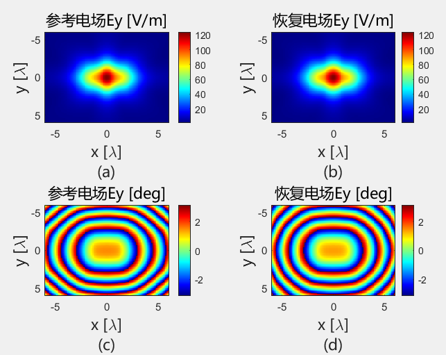
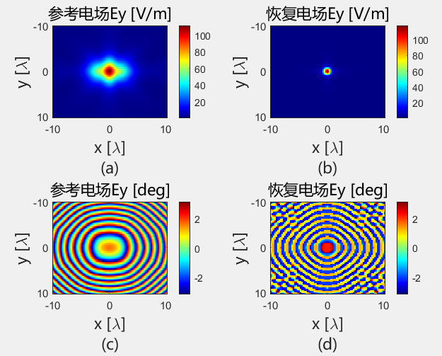
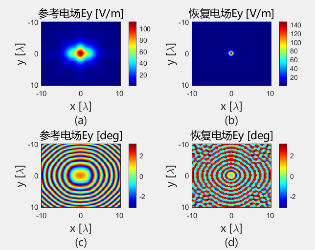
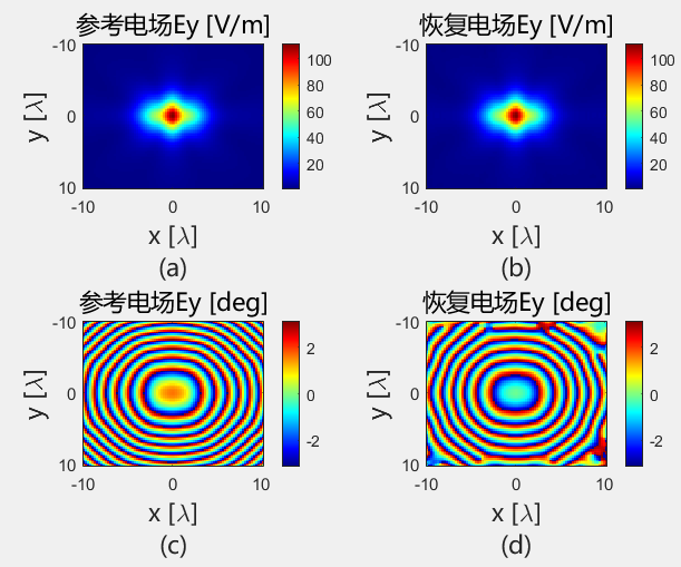
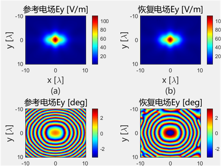
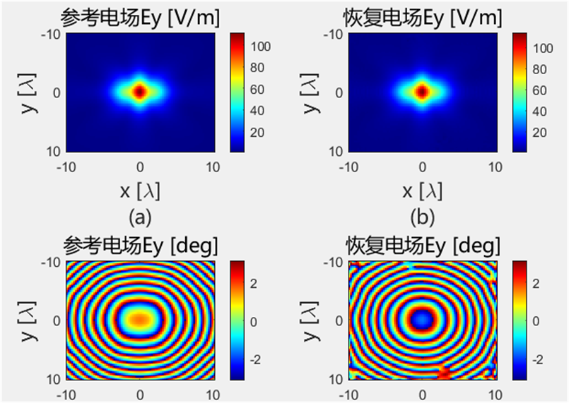
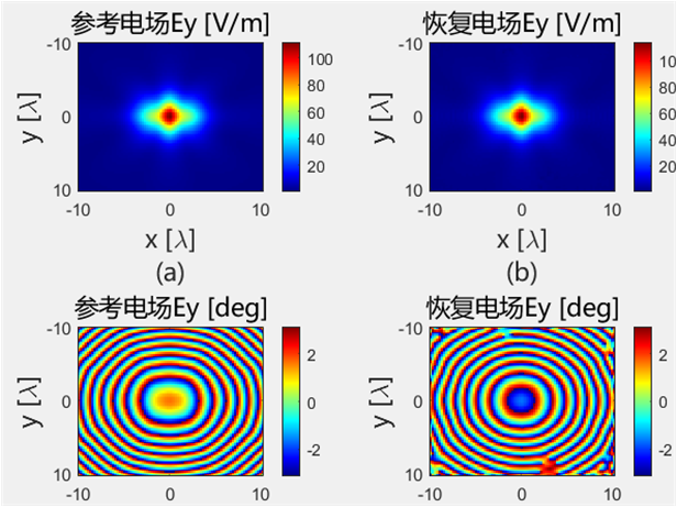
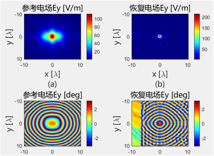
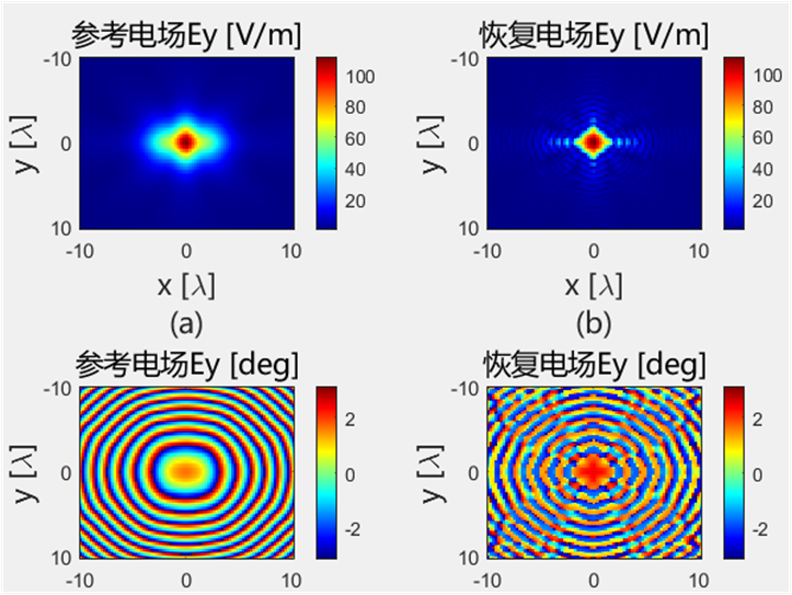
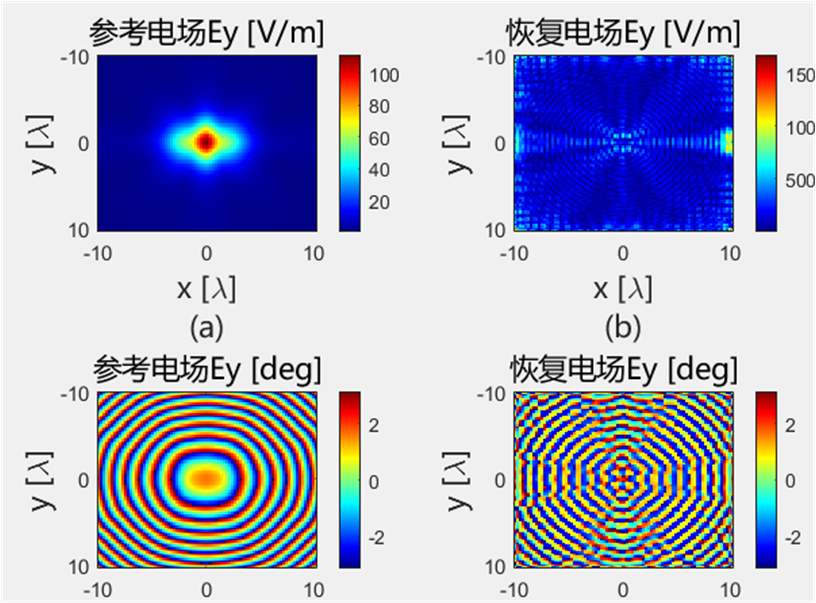
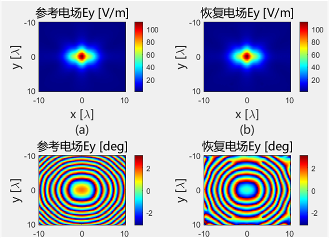
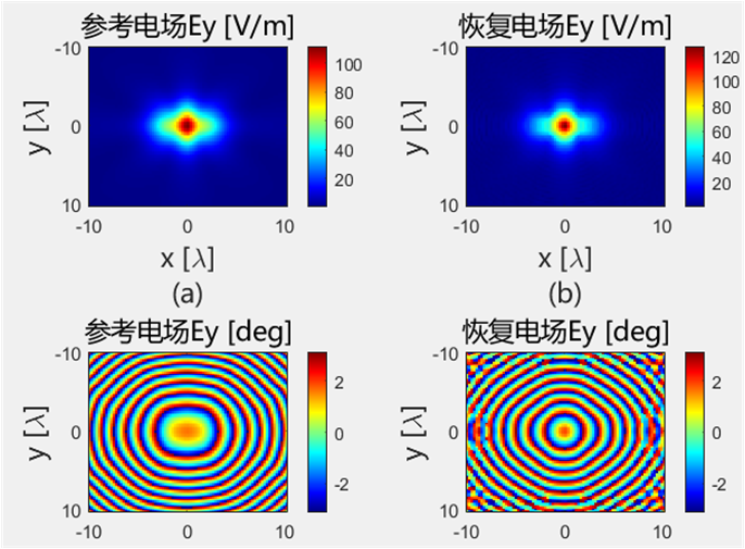
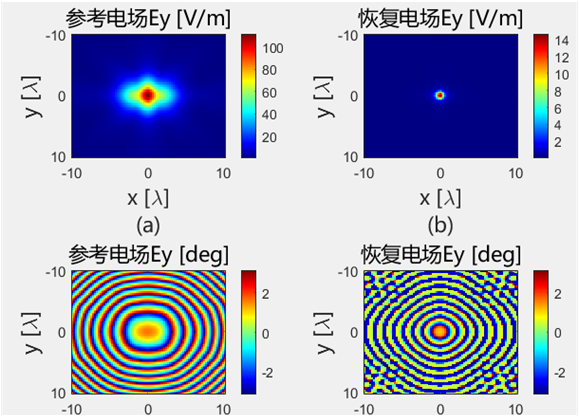
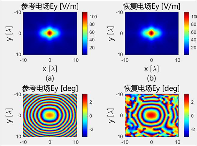
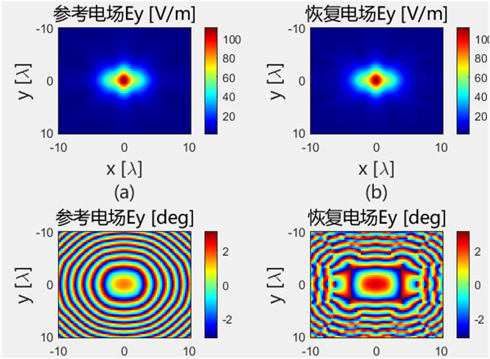
初始化结果对比 下面的是Python代码得到的初始电场幅值和相位:
下面的是Python代码得到的初始电场幅值和相位:
使用初始化结果进行迭代
初始化方法的适配性 使用相同的初始化方法,对得到的初始值使用 PhaseRetrival 工具包里面的14种迭代算法进行处理。
AF / RAF 算法流程:
Amplitude flow Iter = 1000 | IterationTime = 19.554 | Resid = 9.727e-05 | Stepsize = 8.659e-02 Image recovery required 1000 iterations (19.554327 secs)
coordinatedescent Iteration = 1000 | IterationTime = 22.650226 | Residual = 1.109819e-02 Image recovery required 1000 iterations (22.650226 secs)
fienup Iteration = 1000 | IterationTime = 257.996386 | Residual = 2.458595e-03 Image recovery required 1000 iterations (257.996386 secs)
Gerchberg saxton Iteration = 1000 | IterationTime = 267.052254 | Residual = 2.397953e-03 Image recovery required 1000 iterations (267.052254 secs)
kaczmarz Iteration = 1000 | IterationTime = 3.808584 | Residual = 2.201110e-01 Image recovery required 1000 iterations (3.808584 secs)
phasemax Iteration = 1000 | IterationTime = 9.705762 | Residual = 6.121450e-03 Image recovery required 1000 iterations (9.705762 secs)
phaselamp Iteration = 1000 | IterationTime = 15.793961 | Residual = 2.648620e+02 Image recovery required 1000 iterations (15.793961 secs)
raf Iter = 1000 | IterationTime = 14.745 | Resid = 4.072e-05 | Stepsize = 8.634e+02 Image recovery required 1000 iterations (14.745055 secs)
rwf Iter = 1000 | IterationTime = 14.577 | Resid = 1.713e-04 | Stepsize = 4.141e-01 Image recovery required 1000 iterations (14.576618 secs)
sketchycgm Iteration = 1000 | IterationTime = 454.735320 | Residual = 9.969303e-01 Image recovery required 1000 iterations (454.735320 secs)
taf Iter = 1000 | IterationTime = 64.018 | Resid = 4.227e-04 | Stepsize = 9.676e+02 Image recovery required 1000 iterations (64.018318 secs)
twf 有限值不足,无法进行插值。
wirtflow Iter = 1000 | IterationTime = 13.834 | Resid = 6.174e-05 | Stepsize = 1.598e-06 Image recovery required 1000 iterations (13.833875 secs)
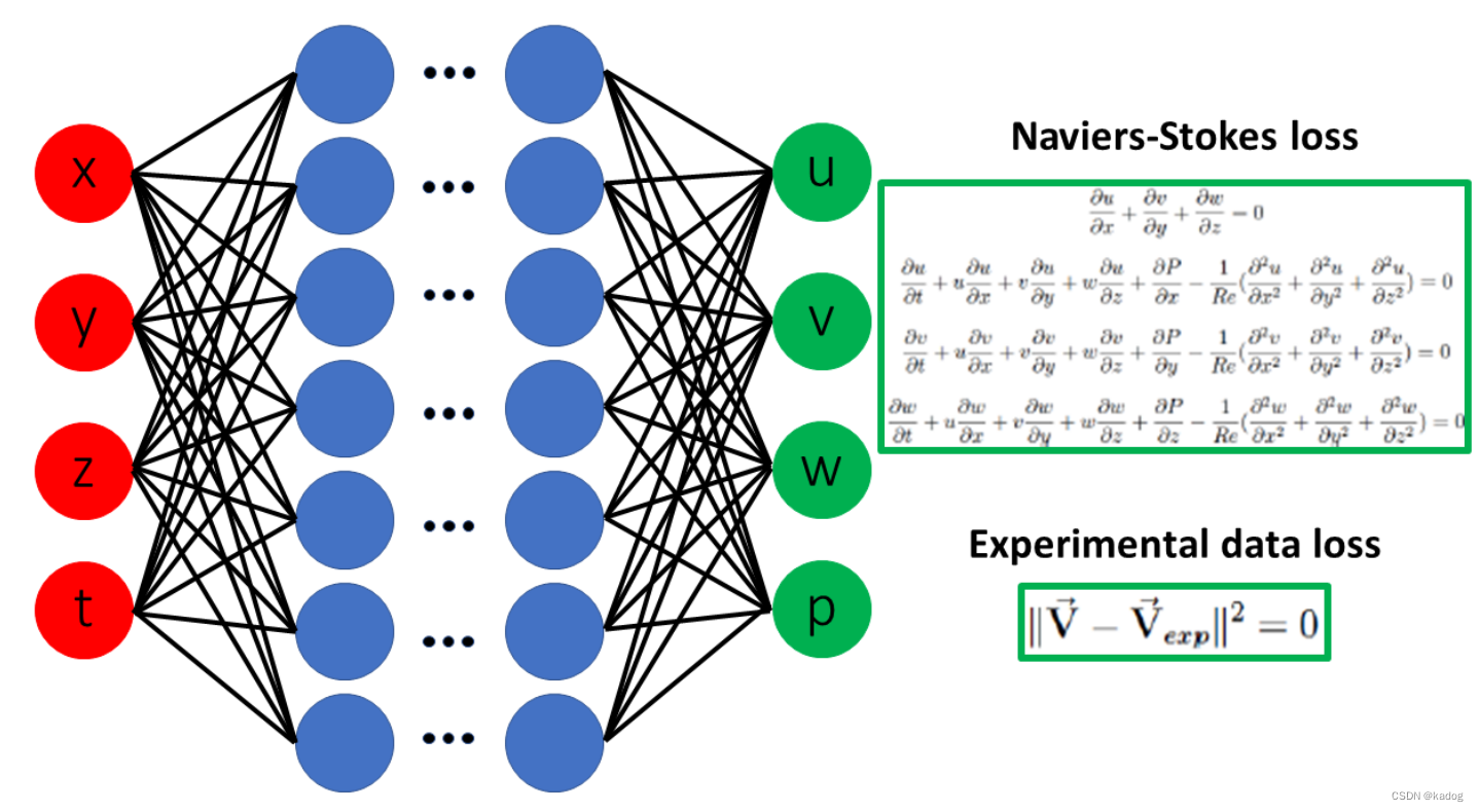
PINN - 物理信息神经网络 PINN - PHYSICS-INFORMED NEURAL NETWORKS
与标准深度学习方法不同,PINN 通过**强制执行控制问题实际物理的偏微分方程 (PDE) **模型的有效性来限制可接受解的空间。
PINN 仅使用一个训练数据集来实现所需的解决方案,从而减轻了替代(即不受物理约束)深度学习方法中所需的大量训练数据集通常带来的负担。
PINN 不需要它预测的逆参数的任何数据,因此它属于无监督学习 。PINN 的这些独特功能对于使用测量场数据或正向模拟生成的合成数据解决逆散射问题非常有益。
PINN 在与前向问题相同的基础上求解高度非线性和色散逆问题,方法是简单地在整体损失函数中增加一个额外的损失项,以最小化偏微分方程及其边界条件的残差 [9]。这些问题通常难以用可用的数学公式来解决。
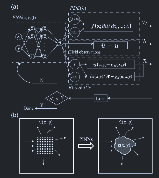
PINN算法 首先构造一个神经将网络的输出$hat{u}(x ; \theta)$作为偏微分方程(PDE)解$u(x)$的替代模型。在这里,我们采用前馈神经网络(FNN),它相对简单,但足以应对大多数偏微分方程问题。$\theta$是一个包含神经网络中所有需要训练的权重和偏差的向量。接下来的关键步骤是约束神经网络的输出$\hat{u}$使其满足偏微分方程以及数据观测值$u$。
这是通过构建损失函数来实现的,该损失函数考虑了对应于偏微分方程、边界条件和初始条件以及场观测值的项。具体来说,我们考虑了以下一个定义在区域$\Omega \subset \mathbb{R}^d$上具有未知参数$\lambda$的偏微分方程问题,其中$x = (x_1, \ldots, x_d)$。
我们考虑的 PDE 问题,实际物理的偏微分方程(PDE) 模型:
我们将$\mathcal{T}_i \subset \Omega$定义为已知 PDE 解$u(\mathbf{x})$的点集。损失函数 定义:
$$
其中$w_f$、$w_b$和$w_i$为权重,$\mathcal{T}_f$、$\mathcal{T}_i$和$\mathcal{T}_b$分别表示来自偏微分方程 、训练数据集 、初始条件和边界条件的残差点集合 。这里,$\mathcal{T}_f \subset \Omega$是一组预定义点,用于衡量神经网络输出$\hat{u}$与 PDE 的匹配程度。$\mathcal{T}_f$可以选择为网格点或随机点。
物理约束项:
$$f(\theta, \lambda; \mathcal{T}_f) = \frac{1}{|\mathcal{T}_f|} \sum {\mathbf{x} \in \mathcal{T}_f} \left| f\left( \mathbf{x}; \frac{\partial \hat{u}}{\partial x_1}, \ldots, \frac{\partial \hat{u}}{\partial x_d}, \frac{\partial^2 \hat{u}}{\partial x_1 \partial x_1}, \ldots, \frac{\partial^2 \hat{u}}{\partial x_1 \partial x_d}; \ldots; \lambda \right) \right|_2^2, \tag{3}
数据匹配项(内部点):
$$i(\theta, \lambda; \mathcal{T}_i) = \frac{1}{|\mathcal{T}_i|} \sum {\mathbf{x} \in \mathcal{T}_i} | \hat{u}(\mathbf{x}) - u(\mathbf{x}) |_2^2, \tag{4}
边界条件项: b(\theta, \lambda; \mathcal{T}_b) = \frac{1}{|\mathcal{T}_b|} \sum {\mathbf{x} \in \mathcal{T}_b} | \mathcal{B}(\hat{u}, \mathbf{x}) |_2^2. \tag{5}
我们通过最小化损失函数$\mathcal{L}(\theta, \lambda)$来优化$\theta$和$\lambda$。需要注意的是,使用 PINNs 的正问题与反问题之间的唯一差别在于,在公式 (2) 中添加了一个额外的损失项$\mathcal{L}_i$。
模型训练时,不仅要最小化数据误差,还要最小化物理信息误差,确保预测结果符合物理定律。
维度 正向问题 逆向问题
已知信息 完整方程+边界/初始条件
部分方程+观测数据
求解目标 物理量场分布
参数、边界或方程形式
驱动因素 物理方程残差主导
数据拟合误差主导
复杂度 相对较低(单优化网络)
较高(联合优化参数与网络)
架构统一性 物理方程残差项占主导(如80%权重)
数据匹配项权重提升(如50%数据损失+50%物理残差)
PINN通过将物理机制显式嵌入神经网络,为正反问题提供了统一的框架,尤其在数据稀疏或高维场景中展现潜力,但其成功依赖于物理方程的合理建模与优化算法的有效性。
案例说明(热传导方程)
正问题 :已知$\alpha$和$f(x,t)$- 网络输出:$u(x,t)$
损失项:PDE残差$|\frac{\partial u}{\partial t} - \alpha \nabla^2 u - f|^2$+ 边界条件
反问题 :未知$\alpha$或$f(x,t)$
网络输出:$u(x,t)$+ $\alpha$(设为可训练标量)
损失项:数据项$|u_{\text{pred}}-u_{\text{obs}}|^2$ + 同上的PDE残差
《用于纳米光学和超材料中逆问题的物理信息神经网络》、Opt Express、2020.4、陈余瑶,卢璐……
采用物理信息神经网络 (PINN) 范式来解决光子超材料和纳米光学技术中代表性的逆散射问题,超越了传统有效介质理论的限制。
物理信息神经网络 (PINN)是最近开发的一个通用框架,用于求解偏微分方程的正向和逆问题 。在本文中,我们提出并开发了 PINN,用于解决与纳米光学和超材料技术直接相关的不同逆散射电磁问题。特别是,我们通过将强大的 PINNs 框架应用于以周期性和非周期性几何形状排列的有限尺寸的散射纳米圆柱体簇,解决了有效介质确定和参数检索的难题。
为了实现目标,使用亥姆霍兹方程约束了物理信息神经网络(PINNs),该方程适用于在 TM 极化激发下具有弱非均匀性的二维(2D)介质:
如图 1(b)示意图所示,手头的问题是通过在有限元方法(FEM)求解散射问题的前向解$u(x, y)$获得的合成数据上训练 PINNs,来反演函数$\varepsilon(x, y)$,这对应于图 1(a)中的未知参数$\lambda$。使用在前向散射有限元模拟中使用 PINNs 预测的介电常数空间轮廓所获得的$\varepsilon(x, y)$验证 PINNs 对介电常数空间轮廓的预测。将得到的电场分布与用于生成训练(合成)散射数据的原始前向有限元模拟的电场分布进行比较。通过计算对应的总场分布的$L^2$误差范数来量化这两个数据集之间的差异。
在本节中,我们训练 PINNs 以预测整个计算域上的介电常数轮廓,因此在这种情况下,我们不需要显式地考虑边界条件的损失项 $\mathcal{T}_b$。
在所有仿真中,我们使用 150 × 150 的空间分辨率对电场进行采样。所使用的 PINN 架构由一个前馈神经网络组成,该网络具有 4 个隐藏层,每个隐藏层中有 64 个神经元。我们使用了双曲正切激活函数,并选择了 Glorot uniform 方法进行权重初始化。训练的学习率设置为$10^{-3}$。最后,我们使用 Adam 方法训练神经网络,并训练 150000 次迭代(epoch),损失值达到$10^{-2}$ 。
多体与多层结构确定性电磁散射理论及其在通信和遥感中的应用 浙江大学、2025.4、P-ANN 算法反演(物理内嵌人工神经网络)、基于相干电磁散射模型的分层土壤物理神经网络反演算法
结合精确散射模型的物理神经网络反演算法(P-ANN)。这也为确定性散射模型在实际物理应用问题,特别是涉及电磁逆问题。分层土壤辐射亮温建模主要通过基于麦克斯韦方程和分层媒质并矢格林函数以及涨落耗散定理推导的相干模型表达。
分层土壤被动遥感的物理神经网络模型
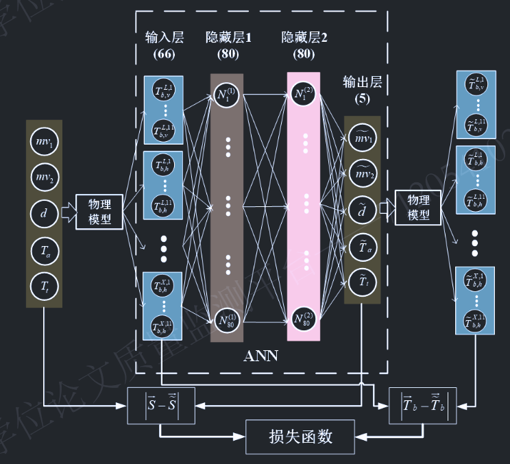
本文所提出的物理内嵌神经网络模型的核心在于,将物理亮温模型 引入到全连接前馈神经网络的损失函数中,以物理约束 和结果约束 双重作用到网络训练和参数反演。本章所有的神经网络构建,训练和测试,均基于MATLAB2023a的深度学习开发库,并遵循与示例类似的风格。P-ANN的框架详细说明如下:
输入层和输出层 :
多频率(L波段、C波段和X波段)、多极化(水平极化和垂直极化)以及 多角度(30:2:50度) 的亮温作为神经网络的输入层。观测角度从30度到50度以2度为间隔选取,因此输入层总计共66个节点。
如前所述的双层土壤的五个土壤参数 (上层湿度,下层湿度,厚度,上层温度,下层温度)作为输出层。
损失函数 :
由土壤参数预测值与真实值 之间的差异($\text{Loss}_0$) 以及其对应的辐射亮温差异 ($\text{Loss}_p$)共同构成:
$$
$$p = \frac{1}{N_0} \sum_{i=1}^{N_0} \left( \left| \overline{T}_{bi}^0 - \widetilde{\overline{T}} {bi}^0 \right| \right)
其中,$|\cdot|$表示 L2 范数(欧几里得范数)的平方,$N_0$为训练数据的样本数。$\overline{S}i^0$和$\tilde{\overline{S}}i^0$分别表示第$i$个采样的真实和预测土壤参数向量,维度均为 5。$\overline{T} {bi}^0$和$\tilde{\overline{T}} {bi}^0$分别表示与$\overline{S}_i^0$和$\tilde{\overline{S}}_i^0$对应的亮温向量,维度均为 66 。需要说明的是,此处使用的变量均为归一化值,以平衡它们在损失函数中的贡献。
训练集,归一化和网络训练 :
在该范围内随机生成5000组 (N0=5000)土壤参数作为训练数据集。随后,通过物理模型计算多频率、多极化和多角度下的对应亮温 ,并将其作为神经网络的输入用于训练过程。
各参数输入网络训练时,需先对输入和输出值进行归一化处理,以消除数据单位和尺度不一致的影响,归一化公式如下:
$$
其中,$s^0$和$T_b^0$分别为归一化后的土壤参数和亮温值,$s_{up}$和$s_{low}$分别为土壤参数的上限和下限。
综合考虑精度和效率,本文在训练过程中采用 L-BFGS 算法(Limited-memory Broyden-Fletcher-Goldfarb-Shanno 算法)作为网络训练的优化算法。
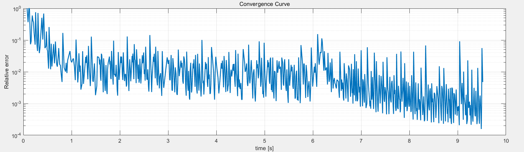
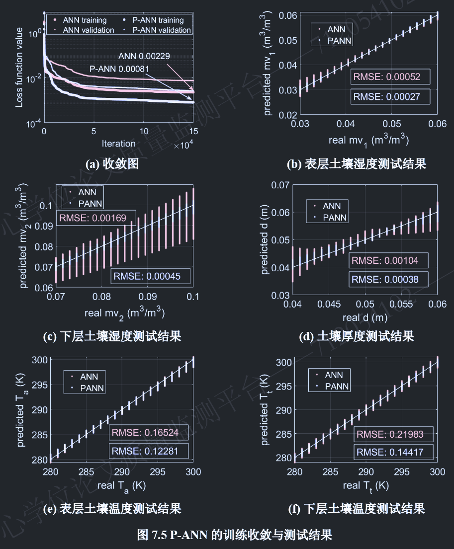
P-ANN在训练过程中的损失函数收敛曲线整体上训练在150,000次 迭代后收敛,步长范数(两次连续迭代之间的步长)和一阶最优性(损失函数梯度的无穷范数)均小于10−5 。在训练过程中,本文还附加验证过程用于评估训练过程中是否出现过拟合现象。验证集的选取为,每个土壤参数均匀采样11个数据点,组合形成115组的数据。验证集每200次迭代评估一次,从图中可以看出,验证集的损失函数值持续下降,未出现过拟合问题。
测试结果
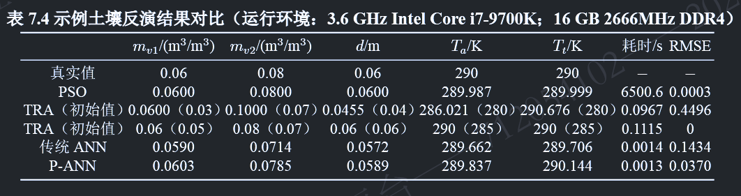
训练完成后,在土壤范围内,每个土壤参数均匀采样21个点 ,将所有可能的参数组合形成总计215组数据作为测试土壤 。对于每组测试土壤参数,使用物理模型计算辐射亮温 ,并将其输入P-ANN模型以预测土壤参数,从而形成测试集。
P-ANN 预测结果与真实值比较如图 7.5 (b)-(d) 所示,结果表明各参数的 P-ANN 反演结果与真实值高度吻合。各反演参数的均方根误差(RMSE)如图中所示。相对而言,与 P-ANN 方法相比,未将物理模型纳入损失函数的传统神经网络的反演性能较差。仅使用预测值与真实值之间的差异(即 Loss0,见公式 7-63)作为损失函数 进行训练的网络,经过相同次数的迭代后,最终损失函数值为 0.00229 ,劣于 P-ANN 方法,如图 7.5 (a) 所示。此外,对于相同的测试集,其预测值与真实值的偏差也较大。特别是下层土壤湿度和土壤厚度的偏差更为明显,如图 7.5 (c) 和 (d) 所示。这两个参数本身由于微波穿透能力问题,就是较为难反演的参数。然而本文提出的 P-ANN 方法由于结合了物理模型在损失函数中,可以有效约束其反演结果 。
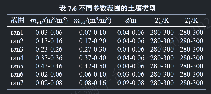
所提出的P-ANN模型在土壤参数范围较小 的情况下获得了好的效果。为了处理更大范围土壤参数的反演问题,一种潜在的策略是采用“分而治之”的方法,即将大土壤参数范围划分为较小范围,并为每个范围训练专用的神经网络,以平衡反演精度和训练成本 。例如,本节中分别在五个不同的参数范围(如表7.6中的ran1-ran5所示)训练了P-ANN模型,并使用相同数量的测试数据评估其反演效果。土壤湿度范围的设定基于现有广泛报道的全国土壤湿度数据集,土壤厚度设定基于电磁波穿透深度。表7.7展示了每个范围的测试结果。P-ANN模型在ran1-ran3范围内表现较好,而在ran4-ran5范围内表现相对较差,尤其是在下层土壤湿度和厚度的反演结果上。这主要是由于高土壤湿度将对应于更高的介电常数,从而限制电磁波的穿透能力。因此在高湿度场景,本质上是难以反演下层相关参数的。这一结论也与其他文献的研究报道一致。需说明,这并非算法本身的问题,而是电磁物理过程固有约束的结果 。
物理神经网络初始化的局部优化算法 - P-ANN 初始化的局部优化算法
当考虑采用优化算法解决上述土壤反演问题时,其目标是找到满足以下条件的最优土壤参数$ilde{s}$:
$$
其中,$N$是观测通道的数量,在本文多通道观测策略下其值为 66(1 个角度 × 2 种极化 × 3 个频率)。$\gamma$代表每个观测通道,$s$是土壤参数向量,本文中长度为 5。
$T_b^{calc}(\gamma,s)$是通道$\gamma$中对应于土壤参数向量$s$的计算亮温,而$T_b^{ex}(\gamma)$是通道$\gamma$中的实测亮温,在本文中通过假设的真实土壤$s$,使用物理模型仿真获得。$\sigma(\gamma)$是权重系数,用于加权不同通道的贡献。在本文中,每个通道的权重系数设为 1 。归一化土壤参数$\tilde{s}^n$与归一化真实值$s^n$ 之间的 RMSE 值被用来衡量反演性能。
考虑到大面积数据反演的高效性,局部优化算法是常用的快速优化算法 。但在使用局部优化算法时,初始值的选取是至关重要的,算法从该初始值,采用梯度下降等技术(如本文中使用的信赖域算法)进行优化。如在上文表 7.4 所展示的两种不同初始值对应的局部优化反演结果,反演过程的最终结果显著依赖于初始值的选取 。随机的初始值选取通常会导致不准确的反演结果,而相对精确的初始值通常能促进优化的快速收敛并产生高精度的反演结果 。
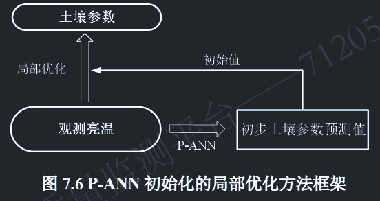
正如人脑通常也提供不精确的推断,我们在上一节的测试也表明,P-ANN的输出事实上也并不是完全准确的,如图7.5所示。然而,这种不精确的结果是相对接近真实值的。因此,通过将P-ANN的结果与局部优化算法结合,将P-ANN的部分准确的输出作为局部优化算法的初始值输入 ,就可以促使局部优化算法在快速梯度下降过程中获得更精确的解。基于这一考虑,我们进一步提出了一种以P-ANN输出为初始值的局部优化方法,其框架如图7.6所示。首先将观测辐射亮温(本文采用仿真获得)输入P-ANN以获得相对准确的土壤参数$s^p$反演结果,然后将其作为信赖域算法的初始值$s^0$进行局部优化反演,以获得更精确的最终反演输出$s^0$。
物理神经网络的可靠性评估
如何确定反演结果的可能误差,或者说反演结果的可靠性,也是在反演中的一个关键的问题。传统的ANN模型通常无法提供此类特征,可以想象,当使用传统ANN反演得到土壤分层参数后,该结果与真实分层参数间误差是无从考证和评估的。然而,物理内嵌的神经网络可以自然地解决这一问题。因为有清晰确定性物理模型后,反演得到的土壤参数可以进一步被计算为对应的微波亮温观测值,其与输入的微波亮温观测之间是可以计算误差的。只需要我们事先拥有土壤参数误差和微波亮温误差之间的统计模型关系,那么依照得到的微波亮温误差就可以评判反演土壤参数结果的误差和可靠性 。而这一误差关系统计模型是可以在P-ANN的测试过程中统计获得的。
如第7.3.3节所述,当使用测试数据测试训练好的神经网络时,可以估计每组反演土壤参数与真实值之间的差异;同时由于引入了物理模型,可以进一步计算反演土壤对应的辐射亮温,从而得到与亮温观测值相比的亮温误差,进而形成土壤参数误差和亮温误差的对应统计关系。这也正是P-ANN相较于传统ANN的另一独特优势。基于大量测试数据,最终可以统计土壤参数误差与对应亮温误差之间的关系。 从而,如上所述,在实际反演过程中,亮温误差易于获取 ,可以根据统计误差关系以一定的置信水平从亮温误差估计土壤参数反演结果的可靠性。
《物理信息神经网络:用于求解涉及非线性偏微分方程的正向和逆向问题的深度学习框架》、Phys、M. Raissi, P. Perdikaris, and G. E. Karniadakis、2019
介绍了物理信息神经网络 – 经过训练以解决监督学习任务的神经网络,同时遵守由一般非线性偏微分方程描述的任何给定物理定律 。在这项工作中,我们展示了我们在解决两大类问题的背景下的发展 :数据驱动的解决方案和数据驱动的偏微分方程发现。通过流体、量子力学、反应扩散系统和非线性浅水波传播中的一系列经典问题证明了所提出的框架的有效性。
在这种小数据制度中,绝大多数最先进的机器学习技术(例如,深度/卷积/递归神经网络)都缺乏稳健性,无法提供任何收敛性保证。乍一看,训练深度学习算法以从几个(可能非常高维的)输入和输出数据对中准确识别非线性映射的任务似乎充其量是天真的。
对于许多与物理和生物系统建模有关的情况,存在大量先验知识,这些知识目前尚未在现代机器学习实践中使用 。无论是支配系统随时间变化的动力学的原则性物理定律,还是一些经过经验验证的规则或其他领域的专业知识,这些先验信息可以充当正则化代理,将可接受解的空间限制在可管理的大小(例如,在可压缩流体动力学问题中,通过丢弃任何违反质量守恒原则的非现实流动解 )。反过来,将此类结构化信息编码到学习算法中会导致算法看到的数据的信息内容放大,使其能够快速将自己引导到正确的解决方案,即使只有几个训练示例可用时也能很好地泛化。
定义$f(t, x)$由方程的左侧给出:
$$神经网络$u(t, x)$和$f(t, x)$之间的共享参数可以通过最小化均方误差损失来学习 :
$$
$$
这里,${(t_i^u, x_i^u, u^i)}_{i=1}^{N_u}$表示$u(t, x)$上的初始 和边界 训练数据,${t_i^f, x_i^f}_{i=1}^{N_f}$指定$f(t, x)$的搭配点。损失$MSE_u$对应于初始和边界数据,而$MSE_f$在一组有限的配置点处强制执行方程$(2)$施加的结构。尽管在以前的研究中已经探索了使用物理定律约束神经网络的类似想法,但在这里,我们使用现代计算工具重新审视它们,并将它们应用于由瞬态非线性偏微分方程描述的更具挑战性的动力学问题。
《量化物理信息神经网络中的总不确定性,以解决正向和逆向随机问题》、Dongkun Zhang, Lu Lu、Journal of Computational Physics、2019
物理信息神经网络 (PINN) 最近成为一种数值求解偏微分方程 (PDE) 的替代方法,无需构建复杂的网格,而是使用简单的实现。特别是,除了解的深度神经网络 (DNN) 之外,还考虑了一个辅助 DNN,它表示 PDE 的残差。然后将残差与给定解数据中的失配相结合,以公式化损失函数。
但由于数据中固有的随机性或 DNN 架构的近似限制,缺乏解决方案的不确定性量化。这里提出了一种新方法,目的是为 DNN 赋予不确定性的两个来源的不确定性量化 ,即参数不确定性和近似不确定性。
当微分方程中的参数表示为随机过程时,我们首先考虑参数不确定性。多个 DNN 旨在通过使用来自稀疏传感器的随机数据来学习其解的任意多项式混沌 (aPC) 扩展的模态函数。然后,我们可以使用经过训练的 DNN 非常有效地从新的传感器测量值中做出预测。
频谱域滤波的作用 Spectral Domain Filtering(频谱域滤波) 是一种在频域中对信号进行处理的技术,通过傅里叶变换将信号从时域/空域转换到频域,然后针对特定频率成分进行增强或抑制。常见的操作包括低通滤波(保留低频)、高通滤波(保留高频)或带通滤波(保留特定频段)。
主要作用
去噪与平滑 :抑制高频噪声(如传感器噪声或干扰)。特征提取 :增强信号中的关键频率成分(如边缘检测中的高频信号)。带宽约束 :限制信号的频率范围以符合物理系统的实际带宽(如光学系统的衍射极限)。先验知识嵌入 :在迭代优化中引入物理约束(如支持域、非负性等)。
在电磁场相位恢复中的必要性 相位恢复的目标是从仅有的强度测量(如光强或电场模值)中重建丢失的相位信息(如相干衍射成像、全息术)。其核心挑战在于该问题是病态(ill-posed) 的,即解不唯一或不稳定。频谱域滤波在此过程中至关重要,原因如下:
抑制噪声与伪影
实际测量中噪声通常存在于高频部分(如散粒噪声、热噪声)。
迭代恢复过程中,噪声会被反复放大,导致解偏离真实值。
频谱域滤波(如低通滤波)可有效抑制高频噪声,提升重建质量。
施加物理约束
电磁场传播受限于物理系统带宽(如光学系统的数值孔径限制)。
超出系统截止频率的成分可能是非物理的,需通过滤波去除(如带通滤波匹配系统传递函数)。
稳定迭代算法
相位恢复算法(如Gerchberg-Saxton、Fienup算法)需在空域和频域交替迭代,施加约束。
频谱域滤波作为频域约束的一部分,可防止算法发散,加速收敛。
解决病态性问题
相位恢复的数学本质是求解非线性方程,需额外约束(如稀疏性、平滑性)。
频谱域滤波通过限制解的频域特性,缩小解空间,使问题适定(well-posed)。
典型应用示例 在相干衍射成像(CDI)中:
实验测得衍射图样(频域强度)。
通过傅里叶变换迭代更新相位,每次迭代中:
频域滤波 :限制频率范围与系统带宽一致,去除超出截止频率的成分。
未滤波的迭代可能导致高频噪声主导,最终重建失败。
在相位恢复算法中频谱域滤波的作用 在相位恢复算法(如 Gerchberg-Saxton(GS)算法 和 Fienup算法 )中,“空域和频域交替迭代,施加约束”是核心操作。这一过程通过反复在两个域(空域和频域)之间传递信号,并施加不同的物理约束,逐步逼近真实的相位解。
角域(角谱)的基本概念: 角域 ,通常称为角谱 ,是指通过傅里叶变换将空间分布的电场或光场分解为不同传播方向的平面波的集合。每个平面波的传播方向由对应的空间频率决定,这些方向的角度分布即构成角谱。
平面波的波矢$k=(k_x,k_y,k_z)$决定了波的传播方向。根据几何关系,传播方向的角度$θ$(例如相对于z轴的倾斜角)满足:
$$\sin\theta = \frac{\sqrt{k_x^2 + k_y^2}}{k} \quad$$
因此,空间频率 $(kx,ky)$直接对应传播角度 。傅里叶变换后的每个点 $(kx,ky)$ 对应一个特定方向的平面波分量,其幅度和相位由傅里叶系数给出。
通过傅里叶变换,复杂的波场被分解为无数个不同方向的平面波叠加。角谱即表示这些平面波的权重分布,反映了波场中各个传播方向的重要性。
角域的物理意义
示例说明 假设一束光垂直照射一个狭缝:
空间域 :狭缝处的电场分布$E(x)$是矩形函数;傅里叶变换 :得到频域的$sinc$函数$\tilde{E}(k_x)$,对应角谱;物理意义 :$sinc$函数的零点间隔表明哪些传播角度(空间频率)被抑制,对应衍射图样的暗条纹。
关键公式 :
$$\text{角谱} \propto \tilde{E}(k_x, k_y), \quad \text{传播角度} \propto \arctan\left(\frac{\sqrt{k_x^2 + k_y^2}}{k_z}\right).$$
模态函数失去正交性 从近场测量中获得远场方向图的经典方法是采用模态展开方法,该方法基于以下事实:适当表面上的场可以表示为一组正交函数的线性组合。
在这种方法中,在测量截断表面上的电场或磁场的切向分量后,利用模态函数的正交性获得模态系数。但是,这些函数在原始表面上是正交的,但在截断表面上不是正交的,因此这些系数的计算是错误的。
这个误差在计算的远场模式中被转化为两种不同的效应。一方面,在某个光谱区域之外,结果完全不可靠。另一方面,由于截断表面边缘处的测量场不连续,该区域内会出现错误的波纹。
因此,整个计算模式始终受到误差的影响,并且无法定义误差完全为零的区域。但是,光谱可靠区域的概念通常用于指代误差不可忽略但较低的区域。其中使用几何光学来计算用于定义可靠区域的最大有效角。
在截断表面上,模态函数失去正交性的原因可以从数学和物理两个层面来理解:
1. 正交性的数学本质 正交性是指两个函数在某个定义域(如无限大表面)上的内积(积分)为零。对于无限大表面上的模态函数(如平面波、球面谐波等),其正交性成立的条件是:
积分范围受限 :积分仅在有限区域$S_{\text{truncated}}$内进行,即:函数截断后的交叠 :截断导致模态函数的“尾部”被切除,原本在无限域中正交的函数可能在有限域内部分重叠,导致内积不为零。
2. 物理机制:场的截断效应
无限表面与有限表面的对比
边缘不连续性 :截断会导致场在边缘处突然截止(类似信号处理中的矩形窗截断),产生高频分量(吉布斯现象)。能量泄漏 :截断后的场无法完整包含原模态的全部能量,不同模态的泄漏能量在有限区域内交叠,破坏了正交性。
3. 具体例子:平面波展开 以平面波展开为例:
无限表面上的正交性 n \cdot \mathbf{r}}$在无限域内正交: {-\infty}^{\infty} e^{j(\mathbf{k}_m - \mathbf{k}_n) \cdot \mathbf{r}} , d\mathbf{r} = \delta(\mathbf{k}_m - \mathbf{k}_n).截断表面上的正交性破坏
4. 实际影响
模态系数计算错误 远场方向图误差
总结
数学层面 :有限积分域破坏了无限域正交性的严格条件。物理层面 :场的截断导致能量泄漏和模态交叠,类似于信号处理中的频谱泄漏现象。
这一现象是近场测量中误差的主要来源,也是定义“光谱可靠区域”的理论基础。


 wechat
 alipay