1
2
3
4
5
6
7
8
9
10
11
12
13
14
15
16
17
18
19
20
21
22
23
24
25
26
27
28
29
30
31
32
33
34
35
36
37
38
39
40
41
42
43
44
45
46
47
48
49
50
51
52
53
54
55
56
57
58
59
60
61
62
63
64
65
66
67
68
69
70
71
72
73
74
75
76
77
78
79
80
81
82
83
84
85
86
87
88
89
| clc
clear all
fc = 1000000;
fm = 1084;
fs = 100000000;
t = 0:1/fs:4/fm;
A0 = 3;
N = length(t);
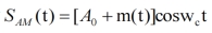
mt = cos(2*pi*fm*t);
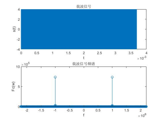
st = 4*cos(2*pi*fc*t);
Sam = (A0 + mt).*st;
Mw = abs(fftshift(fft(mt,N)));
Sw = abs(fftshift(fft(st,N)));
Samw = abs(fftshift((fft(Sam,N))));
fredraw = (-N/2:N/2-1)*(fs/N);
s1 = Sam.*cos(2*pi*fc*t);
s1w = abs(fftshift(fft(s1,N)));
f_bands=[10000,150000];
a = [10,0];
dev = [0.005,0.005];
[N,Wn,beta,ftype] = kaiserord(f_bands,a,dev,fs);
h = fir1(N,Wn,'low',kaiser(N+1,beta));
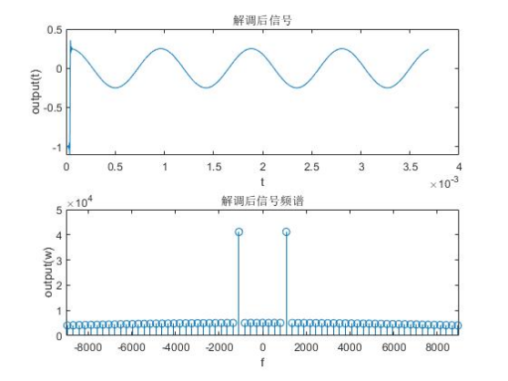
output=filter(h,1,s1)/2-A0;
outputw = abs(fftshift(fft(output)));
figure(1)
subplot(2,1,1)
plot(t,mt)
title('调制信号')
ylabel('m(t)');
xlabel('t');
hold on
subplot(2,1,2)
stem(fredraw,Mw)
title('调制信号频谱')
ylabel('Fm(w)');
xlabel('f');
axis([-9000 9000 0 200000]);
hold on
figure(2)
subplot(2,1,1)
plot(t,st)
title('载波信号')
ylabel('s(t)');
xlabel('t');
hold on
subplot(2,1,2)
stem(fredraw,Sw)
title('载波信号频谱')
ylabel('Fc(w)');
xlabel('f');
axis([-2200000 2200000 0 1000000]);
hold on
figure(3)
subplot(2,1,1)
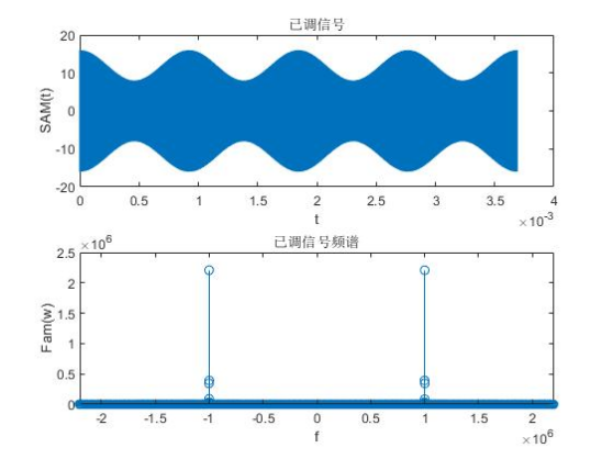
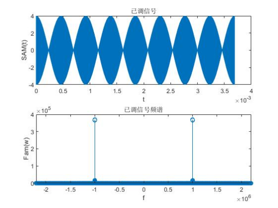
plot(t,Sam)
title('已调信号')
ylabel('SAM(t)');
xlabel('t');
hold on
subplot(2,1,2)
stem(fredraw,Samw)
title('已调信号频谱')
ylabel('Fam(w)');
xlabel('f');
axis([-2200000 2200000 0 2500000]);
hold on
figure(4)
subplot(2,1,1)
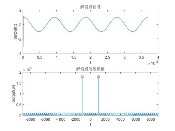
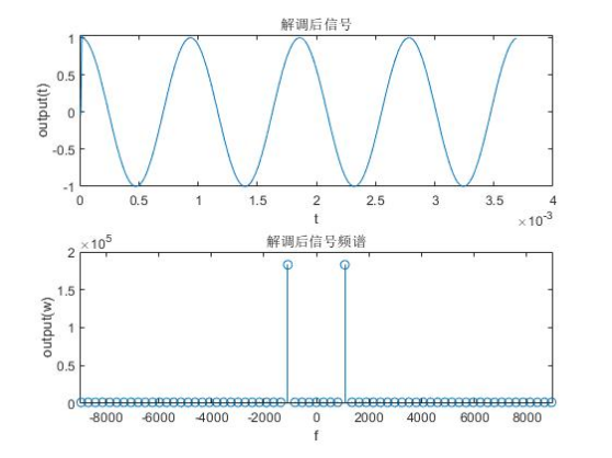
plot(t,output)
title('解调后信号')
ylabel('output(t)');
xlabel('t');
hold on
subplot(2,1,2)
stem(fredraw,outputw)
title('解调后信号频谱')
ylabel('output(w)');
xlabel('f');
axis([-9000 9000 0 200000]);
hold on
|


 wechat
 alipay