非凸优化:综述
A Survey of Non-Convex Optimization
1. Introduction
Optimization is a pervasive discipline that provides the mathematical foundation for decision-making across science and engineering. It seeks to identify an optimal solution from a candidate set by minimizing or maximizing an objective function, often under a set of constraints. The theory of optimization is bisected into two domains: convex and non-convex optimization.
优化是一门无处不在的学科,它为科学和工程领域的决策制定提供了数学基础。它旨在通过最小化或最大化一个目标函数,并常常在一系列约束条件下,从一个候选集合中找出最优解。优化理论被分为两个领域:凸优化和非凸优化。
Convex optimization problems are characterized by a convex objective function and a convex feasible set. They possess a remarkable and powerful property: any locally optimal solution is also globally optimal. This eliminates the ambiguity of local minima and has led to the development of highly efficient, polynomial-time algorithms with robust convergence guarantees.
凸优化问题的特点是其目标函数为凸函数,可行域为凸集。它们拥有一个卓越而强大的特性:任何局部最优解同时也是全局最优解。这消除了局部最小值的模糊性,并催生了具有强大收敛保证的高效多项式时间算法的发展。
In stark contrast, non-convex optimization addresses the more general—and vastly more challenging—class of problems where this convexity assumption is violated. The absence of convexity shatters the guarantee of a unique minimum. The “landscape” of a non-convex function can be exceptionally complex, populated with numerous local minima, maxima, and saddle points, creating a rugged terrain for any optimization algorithm. Finding the global optimum of a general non-convex problem is, in the worst case, computationally intractable and formally classified as NP-hard. This intrinsic difficulty arises from numerous sources, including the combinatorial nature of discrete variables (e.g., in integer programming), non-linear system dynamics, or complex data representations.
与之形成鲜明对比的是,非凸优化处理的是一类更通用——也更具挑战性——的问题,在这些问题中,凸性假设被违背。凸性的缺失打破了全局唯一最小值的保证。非凸函数的“地形”可能异常复杂,遍布着大量的局部最小值、最大值和鞍点,为任何优化算法创造了一片崎岖的地形。在最坏情况下,寻找一个通用非凸问题的全局最优解是计算上不可行的,并被正式归类为NP难问题。这种内在的困难源于多种因素,包括离散变量的组合性质(例如,在整数规划中)、非线性系统动力学或复杂的数据表示。
However, the prevalence of non-convexity in real-world applications has necessitated a paradigm shift. In fields like modern machine learning, the traditional goal of finding the certifiable global optimum is often relaxed. For instance, when training deep neural networks, the objective is less about finding the absolute minimum of the loss function and more about finding a “good” solution—a set of parameters that exhibits strong generalization performance on unseen data. This has spurred intense research into the geometry of non-convex loss functions, leading to concepts like benign landscapes, where most local minima are qualitatively good and saddle points, rather than poor local minima, are the primary bottleneck for optimization. This survey delves into the formulation, algorithmic strategies, and challenges of navigating these complex non-convex landscapes.
然而,非凸性在现实世界应用中的普遍存在,已经催生了一场范式转变。在现代机器学习等领域,寻找可验证的全局最优解这一传统目标常常被放宽。例如,在训练深度神经网络时,目标不再是找到损失函数的绝对最小值,而是找到一个“好的”解——即一组在未见过的数据上表现出强大泛化性能的参数。这激发了对非凸损失函数几何学的深入研究,引出了诸如良性地形 (benign landscapes) 等概念。在这些地形中,大多数局部最小值在质量上都是好的,而鞍点(而非质量差的局部最小值)是优化的主要瓶颈。本综述将深入探讨在这些复杂的非凸地形中进行导航的数学表述、算法策略及所面临的挑战。
2. Mathematical Formulation and Key Concepts
A general non-convex optimization problem, including constraints, is formally stated as:
一个包含约束的通用非凸优化问题,其正式表述如下:
$$
\begin{aligned}
& \min_{x \in \mathbb{R}^n} && f(x) \
& \text{subject to} && g_i(x) \leq 0, \quad i = 1, \dots, m \
& && h_j(x) = 0, \quad j = 1, \dots, p
\end{aligned}
$$
Here, $f(x)$ is the objective function. The functions $g_i(x)$ define the inequality constraints, and $h_j(x)$ define the equality constraints. The set of all points $x$ satisfying these constraints forms the feasible region. The problem is non-convex if $f(x)$ is non-convex, or if any of the constraint functions $g_i(x)$ are non-convex, or if any of the equality constraints $h_j(x)$ are not affine.
这里,$f(x)$ 是目标函数。函数 $g_i(x)$ 定义了不等式约束,而 $h_j(x)$ 定义了等式约束。所有满足这些约束的点 $x$ 的集合构成了**可行域 (feasible region)**。如果目标函数 $f(x)$ 是非凸的,或者任何一个约束函数 $g_i(x)$ 是非凸的,或者任何一个等式约束 $h_j(x)$ 不是仿射函数,那么该问题就是非凸的。
Key Concepts:
关键概念:
Optimality Conditions:
最优性条件 (Optimality Conditions):
First-Order Stationary Point (FOSP): For unconstrained problems, this is a point $x^*$ where the gradient vanishes: $\nabla f(x^*) = 0$.
一阶驻点 (First-Order Stationary Point, FOSP): 对于无约束问题,这是一个梯度为零的点 $x^*$:$\nabla f(x^*) = 0$。
Second-Order Stationary Point (SOSP): A point $x^*$ that is a FOSP and where the Hessian matrix ($\nabla^2 f(x^*)$) is positive semidefinite ($\nabla^2 f(x^*) \succeq 0$). This condition ensures the point is a local minimum.
二阶驻点 (Second-Order Stationary Point, SOSP): 一个点 $x^*$,它既是一阶驻点,并且其海森矩阵 (Hessian matrix) ($\nabla^2 f(x^*)$) 是半正定的 ($\nabla^2 f(x^*) \succeq 0$)。此条件确保该点是一个局部最小值。
Karush-Kuhn-Tucker (KKT) Conditions: For constrained problems, the KKT conditions are the first-order necessary conditions for optimality. They generalize the $\nabla f(x) = 0$ rule and involve both the objective function’s gradient and the constraints’ gradients (via Lagrange multipliers).
KKT 条件 (Karush-Kuhn-Tucker Conditions): 对于有约束问题,KKT条件是满足最优性的一阶必要条件。它们推广了 $\nabla f(x) = 0$ 的规则,并通过拉格朗日乘子将目标函数和约束函数的梯度联系起来。
The Geometry of Non-Convex Landscapes:
非凸地形的几何学:
Saddle Points: A stationary point that is not a local extremum. A strict saddle point is a saddle point where the Hessian matrix has at least one negative eigenvalue. Recent theory suggests that many algorithms (especially those with noise, like SGD) can efficiently escape strict saddle points, but non-strict (degenerate) saddles pose a greater challenge.
鞍点 (Saddle Points): 不是局部极值的驻点。严格鞍点 (strict saddle point) 是指其海森矩阵至少有一个负特征值的鞍点。近期的理论表明,许多算法(尤其是带有噪声的算法,如SGD)可以有效地逃离严格鞍点,但非严格(退化)的鞍点则构成更大的挑战。
Loss Landscape: A term used heavily in deep learning to describe the geometry of the loss function $f(x)$ over the high-dimensional space of model parameters $x$. Understanding this landscape is key.
损失地形 (Loss Landscape): 这个术语在深度学习中被广泛使用,用以描述损失函数 $f(x)$ 在模型参数 $x$ 的高维空间中的几何形状。理解这种地形至关重要。
Basins of Attraction: The set of starting points from which a given local optimization algorithm will converge to the same local minimum. A landscape with wide, “flat” basins is generally considered easier to optimize than one with many narrow, “sharp” basins. Flat minima are often correlated with better generalization.
吸引盆 (Basins of Attraction): 指的是一个点集,从该集合中的任意点出发,一个给定的局部优化算法都会收敛到同一个局部最小值。一个拥有宽而“平坦”吸引盆的地形,通常被认为比一个拥有许多窄而“尖锐”吸引盆的地形更容易优化。平坦的最小值通常与更好的泛化能力相关。
Benign Landscape Hypothesis: A hypothesis suggesting that for certain highly over-parameterized models (like deep neural networks), the loss landscape is “benign” in that (1) most local minima have a value close to the global minimum, and (2) all saddle points are strict, allowing first-order methods to escape them.
良性地形假说 (Benign Landscape Hypothesis): 这是一个假说,它认为对于某些高度过参数化的模型(如深度神经网络),其损失地形是“良性的”,体现在:(1) 大多数局部最小值的值都接近全局最小值;(2) 所有的鞍点都是严格鞍点,从而允许一阶方法逃离它们。
3. Algorithmic Approaches
Algorithms for non-convex optimization must balance the trade-off between computational cost and the quality of the solution found.
非凸优化算法必须在计算成本和所找到解的质量之间进行权衡。
3.1 Local Search Methods
3.1 局部搜索方法
First-Order Methods: These methods only require gradient information.
一阶方法: 这类方法仅需要梯度信息。
Gradient Descent (GD) and its Variants:
梯度下降 (GD) 及其变体:
Momentum: This technique helps accelerate SGD in relevant directions and dampens oscillations. It adds a fraction of the previous update vector to the current one, accumulating a “velocity.”
动量法 (Momentum): 该技术有助于在相关方向上加速SGD并抑制振荡。它将先前更新向量的一部分添加到当前更新中,从而积累“速度”。
Stochastic Gradient Descent (SGD): The cornerstone of large-scale ML. Its inherent noise, arising from mini-batch sampling, acts as a form of regularization and is crucial for escaping sharp local minima and strict saddle points.
随机梯度下降 (SGD): 大规模机器学习的基石。其源于小批量采样的内在噪声,起到了一种正则化的作用,并且对于逃离尖锐的局部最小值和严格鞍点至关重要。
Adaptive Methods (Adam, RMSprop, Adagrad): These algorithms maintain a per-parameter learning rate, adapting based on the history of past gradients. They often converge faster in practice but can sometimes generalize worse than simpler methods like SGD with momentum.
自适应方法 (Adam, RMSprop, Adagrad): 这些算法为每个参数维护一个学习率,并根据过去梯度的历史进行自适应调整。它们在实践中通常收敛更快,但有时其泛化能力可能不如像带Momentum的SGD这样更简单的方法。
Second-Order Methods: These methods utilize the Hessian matrix (second derivatives) to capture the landscape’s curvature.
二阶方法: 这类方法利用海森矩阵(二阶导数)来捕捉地形的曲率信息。
Newton’s Method: This method converges quadratically near a minimum by using a second-order Taylor approximation of the function. The update is $x_{k+1} = x_k - [\nabla^2 f(x_k)]^{-1} \nabla f(x_k)$. However, computing, storing, and inverting the Hessian is prohibitively expensive for high-dimensional problems like deep learning ($O(n^3)$ for inversion).
牛顿法 (Newton’s Method): 该方法通过使用函数的二阶泰勒展开,在最小值附近实现二次收敛。其更新公式为 $x_{k+1} = x_k - [\nabla^2 f(x_k)]^{-1} \nabla f(x_k)$。然而,对于像深度学习这样的高维问题,计算、存储和求逆海森矩阵的成本高得令人望而却步(求逆的计算复杂度为 $O(n^3)$)。
Quasi-Newton Methods (e.g., L-BFGS): These methods avoid explicit Hessian computation by building an approximation of the inverse Hessian using only gradient information from past iterations. L-BFGS (Limited-memory Broyden–Fletcher–Goldfarb–Shanno) is a popular choice for medium-scale problems.
拟牛顿法 (Quasi-Newton Methods, 如 L-BFGS): 这类方法通过仅使用过去迭代的梯度信息来构建海森矩阵逆的近似,从而避免了显式计算海森矩阵。L-BFGS(限域Broyden–Fletcher–Goldfarb–Shanno)是中等规模问题的热门选择。
3.2 Global Search and Approximation Strategies
3.2 全局搜索与近似策略
Heuristic and Stochastic Methods: These methods employ randomness to explore the search space broadly.
启发式与随机方法: 这类方法利用随机性来广泛地探索搜索空间。
Simulated Annealing, Genetic Algorithms, Particle Swarm Optimization: (As described previously).
模拟退火、遗传算法、粒子群优化: (如前所述)。
Bayesian Optimization: A powerful model-based approach for derivative-free optimization of expensive black-box functions. It builds a probabilistic surrogate model (often a Gaussian Process) of the objective function and uses an acquisition function to intelligently decide where to sample next, balancing exploration and exploitation. It is very effective for hyperparameter tuning.
贝叶斯优化 (Bayesian Optimization): 一种强大的、基于模型的方法,用于对昂贵的黑箱函数进行无导数优化。它为目标函数建立一个概率性的代理模型 (surrogate model)**(通常是高斯过程),并使用一个采集函数 (acquisition function)** 来智能地决定下一个采样点,以平衡探索和利用。它在超参数调优方面非常有效。
Deterministic Global Methods and Relaxations: These aim for provable guarantees.
确定性全局方法与松弛技术: 这类方法旨在提供可证明的保证。
Branch and Bound: (As described previously). Its effectiveness hinges on the ability to compute tight lower bounds on the objective function over sub-regions, often via convex relaxation.
分支定界法: (如前所述)。其有效性取决于能否通过凸松弛 (convex relaxation) 等方法,在子区域上计算出目标函数的紧密下界。
Convex Relaxation: This is a powerful technique where a hard non-convex problem is replaced by a related but tractable convex problem (the “relaxation”). For example, Semidefinite Programming (SDP) relaxations are used for quadratically constrained quadratic programs. The solution to the relaxation provides a bound on, and sometimes can be used to recover a solution for, the original problem.
凸松弛: 这是一种强大的技术,它将一个困难的非凸问题替换为一个相关但易于处理的凸问题(即“松弛”问题)。例如,半定规划 (SDP) 松弛被用于求解二次约束二次规划问题。松弛问题的解为原问题提供了一个界限,有时甚至可以用来恢复原问题的解。
Sequential Convex Programming (SCP): This iterative method solves a non-convex problem by approximating it with a sequence of convex subproblems at each step.
序列凸规划 (Sequential Convex Programming, SCP): 这种迭代方法通过在每一步用一系列的凸子问题来近似求解非凸问题。
4. Key Challenges and Theoretical Aspects
Lack of Convergence Guarantees: For most non-convex problems, local search algorithms are only guaranteed to converge to a stationary point, not necessarily a local minimum, and certainly not the global minimum. Proving convergence to even a local minimum is often difficult.
缺乏收敛保证: 对于大多数非凸问题,局部搜索算法仅能保证收敛到一个驻点,而不一定是局部最小值,更不用说是全局最小值。即使是证明收敛到局部最小值也常常很困难。
The Problem of Saddle Points: In high-dimensional spaces, saddle points are exponentially more numerous than local minima. First-order methods like Gradient Descent can get stuck or severely slow down near them. More sophisticated methods that incorporate second-order information or noise (like SGD) are better at escaping saddle points.
鞍点问题: 在高维空间中,鞍点的数量比局部最小值的数量要多出指数级别。像梯度下降这样的一阶方法可能会在鞍点附近被困住或严重减速。包含二阶信息或噪声(如SGD)的更复杂方法能更好地逃离鞍点。
High Dimensionality: The “curse of dimensionality” makes searching the solution space exponentially more difficult as the number of variables ($n$) grows. This is a major challenge in applications like deep learning, where $n$ can be in the billions.
高维度: “维度灾难”使得随着变量数量($n$)的增加,搜索解空间的难度呈指数级增长。这在深度学习等应用中是一个主要挑战,因为 $n$ 的数量可以达到数十亿。
Choosing Hyperparameters: The performance of many algorithms (e.g., learning rate in GD, temperature schedule in simulated annealing) is highly sensitive to the choice of hyperparameters. Finding good hyperparameters can be a difficult meta-optimization problem in itself.
超参数选择: 许多算法的性能(例如,GD中的学习率、模拟退火中的温度调度)对超参数的选择高度敏感。寻找好的超参数本身就是一个困难的元优化问题。
5. Applications
Non-convex optimization is ubiquitous in science and engineering.
非凸优化在科学和工程领域无处不在。
Machine Learning and Deep Learning: This is the most prominent application area today. Training a neural network involves minimizing a non-convex loss function over the network’s weights. Other ML problems like matrix factorization and clustering are also non-convex.
机器学习与深度学习: 这是当今最突出的应用领域。训练神经网络涉及在网络权重上最小化一个非凸的损失函数。其他机器学习问题,如矩阵分解和聚类,也是非凸的。
Robotics: Problems such as trajectory planning and inverse kinematics require optimizing non-convex functions to find feasible and optimal paths.
机器人学: 诸如轨迹规划和逆运动学等问题需要优化非凸函数以找到可行且最优的路径。
Engineering Design: Optimizing the shape of an aircraft wing for minimal drag or designing a complex circuit for maximal performance are non-convex problems.
工程设计: 优化机翼形状以实现最小阻力,或设计复杂电路以获得最高性能,这些都是非凸问题。
Computational Biology: Protein folding, the problem of predicting a protein’s 3D structure from its amino acid sequence, is a notoriously difficult non-convex optimization problem.
计算生物学: 蛋白质折叠,即根据氨基酸序列预测蛋白质三维结构的问题,是一个极其困难的非凸优化问题。
Operations Research: Problems like facility location with non-linear costs or complex scheduling often lead to non-convex integer programming problems.
运筹学: 诸如具有非线性成本的设施选址或复杂的调度问题,通常会导致非凸整数规划问题。
6. Conclusion and Future Directions
Non-convex optimization has transitioned from a theoretical challenge to an indispensable tool for solving some of the most important problems of our time. While local search methods like SGD and Adam have achieved remarkable empirical success, especially in deep learning, our theoretical understanding of why they work so well is still evolving.
非凸优化已经从一个理论上的挑战,转变为解决我们这个时代一些最重要问题的不可或缺的工具。尽管像SGD和Adam这样的局部搜索方法取得了显著的实践成功(尤其是在深度学习领域),但我们对于它们为何如此有效的理论理解仍在发展之中。
Future research will likely focus on:
未来的研究可能会集中在以下几个方面:
Developing more principled and scalable global optimization algorithms.
开发更具原则性、可扩展性更强的全局优化算法。
Gaining a deeper understanding of the loss landscapes of neural networks to design better optimizers.
更深入地理解神经网络的损失函数“地形”, 以此设计出更好的优化器。
Creating algorithms with stronger theoretical guarantees that can provably escape saddle points and find “good” local minima efficiently.
创建具有更强理论保证的算法, 这些算法可以被证明能有效逃离鞍点并找到“好的”局部最小值。
Automating hyperparameter tuning to make algorithms more robust and easier to use.
自动化超参数调优, 使算法更加鲁棒且易于使用。
In summary, non-convex optimization remains a vibrant, challenging, and rapidly advancing field at the heart of modern data science and artificial intelligence.
总而言之,非凸优化仍然是一个充满活力、富有挑战且发展迅速的领域,它正处于现代数据科学和人工智能的核心位置。
Solving Most Systems of Random Quadratic Equations
Abstract
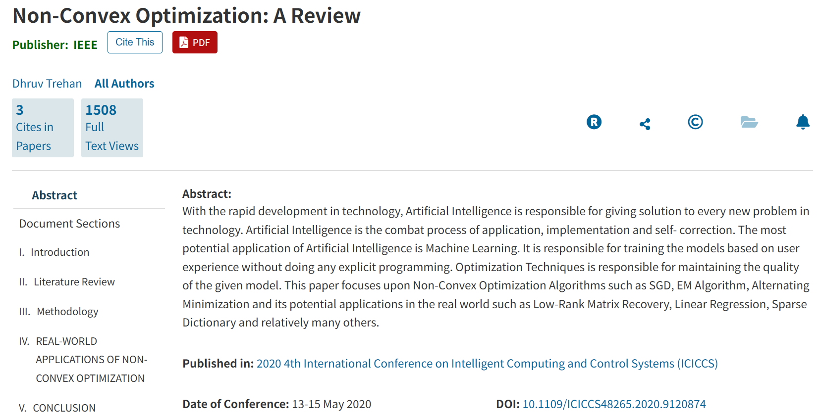
This paper deals with finding an $ n $-dimensional solution $ x $ to a system of quadratic equations $ y_i = |\langle a_i, x \rangle|^2 $, $ 1 \leq i \leq m $, which in general is known to be NP-hard. We put forth a novel procedure, that starts with a weighted maximal correlation initialization obtainable with a few power iterations, followed by successive refinements based on iteratively reweighted gradient-type iterations. The novel techniques distinguish themselves from prior works by the inclusion of a fresh (re)weighting regularization. For certain random measurement models, the proposed procedure returns the true solution $ x $ with high probability in time proportional to reading the data ${(a_i; y_i)}_{1 \leq i \leq m}$, provided that the number $ m $ of equations is some constant $ c > 0 $ times the number $ n $ of unknowns, that is, $ m \geq cn $. Empirically, the upshots of this contribution are:
本文研究如何求解n维解向量$ x $满足二次方程组$ y_i = |\langle a_i, x \rangle|^2 $($ 1 \leq i \leq m $)的问题——该问题在一般情况下被证明是NP难解的。我们提出了一种创新方法:首先通过少量幂迭代获得加权最大相关性初始解,随后基于迭代重加权梯度类方法进行逐步优化。该技术的核心创新在于引入了一种全新的(重)加权正则化策略。对于某些随机测量模型,当方程数$ m $与未知量数$ n $满足$ m \geq cn $(其中$ c > 0 $为常数)时,所提方法能以与数据读取时间${(a_i; y_i)}_{1 \leq i \leq m}$成正比的复杂度,高概率地恢复真实解$ x $。实验结果表明:
perfect signal recovery in the high-dimensional regime given only an information-theoretic limit number of equations;
(near-)optimal statistical accuracy in the presence of additive noise.
在高维场景下,仅需信息论极限数量的方程即可实现完美信号重建;
在加性噪声存在时达到(接近)最优统计精度。
Extensive numerical tests using both synthetic data and real images corroborate its improved signal recovery performance and computational efficiency relative to state-of-the-art approaches.
通过合成数据和真实图像的广泛测试,本方法在信号恢复性能和计算效率方面均显著优于现有先进技术。
1 Introduction
One is often faced with solving quadratic equations of the form $y_i = |\langle a_i, x \rangle|^2$, or equivalently,
$$
\psi_i = |\langle a_i, x \rangle|, \quad 1 \leq i \leq m
$$
where $x \in \mathbb{R}^n / \mathbb{C}^n$ (hereafter, symbol “$A/B$” denotes either $A$ or $B$) is the wanted unknown $n \times 1$ vector, while given observations $\psi_i$ and feature vectors $a_i \in \mathbb{R}^n / \mathbb{C}^n$ that are collectively stacked in the data vector $\psi := [\psi_i]_{1 \leq i \leq m}$ and the $m \times n$ sensing matrix $A := [a_i]_{1 \leq i \leq m}$, respectively.
我们经常需要求解形如$y_i = |\langle a_i, x \rangle|^2$的二次方程组,其等价形式为:
$$
\psi_i = |\langle a_i, x \rangle|, \quad 1 \leq i \leq m
$$
其中$x \in \mathbb{R}^n / \mathbb{C}^n$(后文符号”$A/B$”表示$A$或$B$)是待求的$n \times 1$未知向量,而给定的观测值$\psi_i$和特征向量$a_i \in \mathbb{R}^n / \mathbb{C}^n$分别构成数据向量$\psi := [\psi_i]_{1 \leq i \leq m}$和感知矩阵$A := [a_i]_{1 \leq i \leq m}$。
Put differently, given information about the (squared) modulus of the inner products of the signal vector $x$ and several known design vectors $a_i$, can one reconstruct exactly (up to a global phase factor) $x$, or alternatively, the missing phase of $\langle a_i, x \rangle$.
换句话说,当已知信号向量$x$与若干已知设计向量$a_i$内积的(平方)模量时,能否精确重建$x$(至多相差一个全局相位因子),或者等价地恢复$\langle a_i, x \rangle$的缺失相位?
In fact, much effort has been devoted to determining the number of such equations necessary and/or sufficient for the uniqueness of the solution $x$; see e.g., [1, 8]. It has been proved that $m \geq 2n - 1$ ($m \geq 4n - 4$) generic$^1$ (which includes the case of random vectors) real (complex) vectors $a_i$ are sufficient for uniquely determining an $n$-dimensional real (complex) vector $x$ [1, Theorem 2.8], [8], while in the real case $m = 2n - 1$ is shown also necessary [1]. In this sense, the number $m = 2n - 1$ of equations as in (1) can be regarded as the information-theoretic limit for such a quadratic system to be uniquely solvable.
事实上,已有大量研究致力于确定保证解$x$唯一性所需方程数量的必要/充分条件(参见[1,8])。已证明对于实(复)向量$a_i$,当$m \geq 2n - 1$($m \geq 4n - 4$)时,泛型情况$^1$(包含随机向量情形)足以唯一确定n维实(复)向量$x$[1, 定理2.8], [8],而在实数情形下$m = 2n - 1$也被证明是必要条件[1]。因此,(1)式中方程数量$m = 2n - 1$可视为该二次系统具有唯一解的信息论极限。
Prior contributions
Following the least-squares (LS) criterion (which coincides with the maximum likelihood (ML) one assuming additive white Gaussian noise), the problem of solving quadratic equations can be naturally recast as an empirical loss minimization
根据最小二乘(LS)准则(在加性高斯白噪声假设下与最大似然(ML)准则一致),求解二次方程组的问题可以自然地转化为经验损失最小化问题:
$$
\underset{\boldsymbol{z}\in\mathbb{R}^{n}}{\text{minimize}} \quad L(\boldsymbol{z}):=\frac{1}{m}\sum_{i=1}^{m}\ell(\boldsymbol{z}; \psi_{i}/y_{i})
$$
where one can choose to work with the amplitude-based loss $\ell(\boldsymbol{z};\psi_{i}):=(\psi_{i}-|\langle\boldsymbol{a}{i},\boldsymbol{z}\rangle|)^{2}/2$ [28, 30], or the intensity-based one $\ell(\boldsymbol{z};y{i}):=(y_{i}-|\langle\boldsymbol{a}{i},\boldsymbol{z}\rangle|^{2})^{2}/2$ [3], and its related Poisson likelihood $\ell(\boldsymbol{z};y{i}):=y_{i}\log(|\langle\boldsymbol{a}{i},\boldsymbol{z}\rangle|^{2})-|\langle\boldsymbol{a}{i},\boldsymbol{z}\rangle|^{2}$ [7]. Either way, the objective functional $L(\boldsymbol{z})$ is nonconvex; hence, it is generally NP-hard and computationally intractable to compute the ML or LS estimate.
可选择使用基于振幅的损失函数$\ell(\boldsymbol{z};\psi_{i}):=(\psi_{i}-|\langle\boldsymbol{a}{i},\boldsymbol{z}\rangle|)^{2}/2$[28,30],基于强度的损失函数$\ell(\boldsymbol{z};y{i}):=(y_{i}-|\langle\boldsymbol{a}{i},\boldsymbol{z}\rangle|^{2})^{2}/2$[3],或相关的泊松似然函数$\ell(\boldsymbol{z};y{i}):=y_{i}\log(|\langle\boldsymbol{a}{i},\boldsymbol{z}\rangle|^{2})-|\langle\boldsymbol{a}{i},\boldsymbol{z}\rangle|^{2}$[7]。无论哪种情况,目标函数$L(\boldsymbol{z})$都是非凸的,因此计算ML或LS估计通常是NP难问题且计算上难以处理。
Minimizing the squared modulus-based LS loss in (2), several numerical polynomial-time algorithms have been devised via convex programming for certain choices of design vectors $\boldsymbol{a}_{i}$ [4, 25]. Such convex paradigms first rely on the matrix-lifting technique to express all squared modulus terms into linear ones in a new rank-1 matrix variable, followed by solving a convex semi-definite program (SDP) after dropping the rank constraint. It has been established that perfect recovery and (near-)optimal statistical accuracy are achieved in noiseless and noisy settings respectively with an optimal-order number of measurements [4]. In terms of computational efficiency however, such lifting-based convex approaches entail storing and solving for an $n\times n$ semi-definite matrix from $m$ general SDP constraints, whose computational complexity in the worst case scales as $n^{4.5}\log{1/\epsilon}$ for $m\approx n$ [25], which is not scalable. Another recent line of convex relaxation [12, 13] reformulated the problem of phase retrieval as that of sparse signal recovery, and solved a linear program in the natural parameter vector domain. Although exact signal recovery can be established assuming an accurate enough anchor vector, its empirical performance is in general not competitive with state-of-the-art phase retrieval approaches.
为最小化(2)式中基于平方模的LS损失,针对特定设计向量$\boldsymbol{a}_{i}$[4,25],已开发出几种基于凸规划的数值多项式时间算法。这类凸范式首先通过矩阵提升技术将所有平方模项表示为新秩-1矩阵变量中的线性项,然后通过放弃秩约束求解凸半定规划(SDP)。研究证明[4],在无噪声和有噪声环境下,使用最优阶数量的测量可分别实现完美恢复和(接近)最优统计精度。然而就计算效率而言,这类基于提升的凸方法需要存储并求解来自$m$个一般SDP约束的$n×n$半定矩阵,在最坏情况下(当$m≈n$时)计算复杂度为$n^{4.5}\log{1/\epsilon}$[25],不具备可扩展性。另一类近期提出的凸松弛方法[12,13]将相位恢复问题重新表述为稀疏信号恢复问题,并在自然参数向量域中求解线性规划。虽然可以在假设足够精确的锚向量的情况下建立精确信号恢复的理论保证,但其实际性能通常无法与最先进的相位恢复方法相媲美。
Recent proposals advocate suitably initialized iterative procedures for coping with certain nonconvex formulations directly; see e.g., algorithms abbreviated as AltMinPhase, (R/P)WF, (M)TWF, (S)TAF [16, 3, 7, 26, 28, 27, 30, 22, 6, 24], as well as a prox-linear algorithm [9]. These nonconvex approaches operate directly upon vector optimization variables, thus leading to significant computational advantages over their convex counterparts. With random features, they can be interpreted as performing stochastic optimization over acquired examples ${({\boldsymbol{a}}{i};\psi{i}/y_{i})}{1\leq i\leq m}$ to approximately minimize the population risk functional $\overline{L}(\boldsymbol{z}):=\mathbb{E}{({\boldsymbol{a}}{i},\psi{i}/y_{i})}[\ell(\boldsymbol{z};\psi_{i}/y_{i})]$. It is well documented that minimizing nonconvex functionals is generally intractable due to existence of multiple critical points [17]. Assuming Gaussian sensing vectors however, such nonconvex paradigms can provably locate the global optimum, several of which also achieve optimal (statistical) guarantees. Specifically, starting with a judiciously designed initial guess, successive improvement is effected by means of a sequence of (truncated) (generalized) gradient-type iterations given by
近期研究主张采用适当初始化的迭代程序直接处理某些非凸问题,如AltMinPhase、(R/P)WF、(M)TWF、(S)TAF等算法[16,3,7,26,28,27,30,22,6,24]以及近端线性算法[9]。这些非凸方法直接在向量优化变量上操作,相比凸方法具有显著计算优势。对于随机特征,可将其解释为在采集样本${({\boldsymbol{a}}{i};\psi{i}/y_{i})}{1\leq i\leq m}$上执行随机优化以近似最小化总体风险泛函$\overline{L}(\boldsymbol{z}):=\mathbb{E}{({\boldsymbol{a}}{i},\psi{i}/y_{i})}[\ell(\boldsymbol{z};\psi_{i}/y_{i})]$。文献充分证明[17],由于存在多个临界点,最小化非凸泛函通常是难以处理的。然而对于高斯感知向量,这类非凸范式可证明能找到全局最优解,其中若干方法还能达到最优(统计)保证。具体而言,从精心设计的初始猜测出发,通过以下(截断)(广义)梯度型迭代序列实现逐步改进:
$$
z^{t+1}:=z^{t}-\frac{\mu^{t}}{m}\sum_{i\in\mathcal{T}^{t+1}}\nabla\ell_{i}(z^{t};\psi_{i}/y_{i}),\quad t=0,,1,,\dots
$$
where $z^{t}$ denotes the estimate returned by the algorithm at the $t$-th iteration, $\mu^{t}>0$ is learning rate that can be pre-selected or found via e.g., the backtracking line search strategy, and $\nabla\ell(z^{t},\psi_{i}/y_{i})$ represents the (generalized) gradient of the modulus- or squared modulus-based LS loss evaluated at $z^{t}$. Here, $\mathcal{T}^{t+1}$ denotes some time-varying index set signifying the per-iteration gradient truncation.
其中$z^{t}$表示算法第$t$次迭代返回的估计值,$\mu^{t}>0$是可预设或通过回溯线搜索策略确定的学习率,$\nabla\ell(z^{t},\psi_{i}/y_{i})$表示在$z^{t}$处评估的基于模或平方模的LS损失的(广义)梯度。$\mathcal{T}^{t+1}$表示随时间变化的索引集,用于标识每次迭代的梯度截断。
Although they achieve optimal statistical guarantees in both noiseless and noisy settings, state-of-the-art (convex and nonconvex) approaches studied under Gaussian designs, empirically require stable recovery of a number of equations (several) times larger than the information-theoretic limit [7, 3, 30]. As a matter of fact, when there are numerously enough measurements (on the order of $n$ up to some polylog factors), the squared modulus-based LS functional admits benign geometric structure in the sense that [23]: i) all local minimizers are also global; and, ii) there always exists a negative directional curvature at every saddle point. In a nutshell, the grand challenge of tackling systems of random quadratic equations remains to develop algorithms capable of achieving perfect recovery and statistical accuracy when the number of measurements approaches the information limit.
尽管在无噪声和有噪声环境下都能达到最优统计保证,但在高斯设计下研究的最先进(凸和非凸)方法,实际需要比信息论极限多数倍的方程才能实现稳定恢复[7,3,30]。事实上,当测量数量足够多(达到$n$乘以某些多对数因子量级)时,基于平方模的LS泛函具有良性几何结构[23]:i)所有局部极小值也是全局的;ii)每个鞍点处都存在负方向曲率。简而言之,解决随机二次方程组的重大挑战仍然是开发当测量数量接近信息极限时仍能实现完美恢复和统计精度的算法。
This work
Building upon but going beyond the scope of the aforementioned nonconvex paradigms, the present paper puts forward a novel iterative linear-time scheme, namely, time proportional to that required by the processor to scan all the data ${(a_{i};\psi_{i})}_{1\leq i\leq m}$, that we term reweighted amplitude flow, and henceforth, abbreviate as RAF.
基于前述非凸范式并加以拓展,本文提出了一种新颖的线性时间迭代方案——其计算时间与处理器扫描全部数据${(a_{i};\psi_{i})}_{1\leq i\leq m}$所需时间成正比,我们称之为重加权振幅流(Reweighted Amplitude Flow),简称RAF。
Our methodology is capable of solving noiseless random quadratic equations exactly, yielding an estimate of (near)-optimal statistical accuracy from noisy modulus observations. Exactness and accuracy hold with high probability and without extra assumption on the unknown signal vector $\boldsymbol{x}$, provided that the ratio $m/n$ of the number of equations to that of the unknowns is larger than a certain constant.
该方法能够精确求解无噪随机二次方程,并从含噪模观测中产生(接近)最优统计精度的估计。当方程数与未知量之比$m/n$超过某常数时,解的精确性和准确性均以高概率成立,且无需对未知信号向量$\boldsymbol{x}$施加额外假设。
Empirically, our approach is shown able to ensure exact recovery of high-dimensional unstructured signals given a minimal number of equations, where $m/n$ in the real case can be as small as $2$.
实验表明,本方法在实数情形下仅需最少方程数($m/n$可低至2)即可确保高维非结构化信号的精确恢复。
The new twist here is to leverage judiciously designed yet conceptually simple (re)weighting regularization techniques to enhance existing initializations and also gradient refinements.
本研究的创新点在于巧妙设计概念简洁的(重)加权正则化技术,以改进现有初始化方法和梯度优化过程。
An informal depiction of our RAF methodology is given in two stages as follows, with rigorous details deferred to Section 3:
RAF方法的非正式描述分为两个阶段(严格细节见第3节):
S1) Weighted maximal correlation initialization: Obtain an initializer $\boldsymbol{z}^{0}$ maximally correlated with a carefully selected subset $\mathcal{S}\subsetneq\mathcal{M}:={1,2,\dots,m}$ of feature vectors $\boldsymbol{a}{i}$, whose contributions toward constructing $\boldsymbol{z}^{0}$ are judiciously weighted by suitable parameters ${w{i}^{0}>0}_{i\in\mathcal{S}}$.
S1) 加权最大相关初始化: 获取与特征向量$\boldsymbol{a}{i}$的精选子集$\mathcal{S}\subsetneq\mathcal{M}:={1,2,\dots,m}$具有最大相关性的初始估计$\boldsymbol{z}^{0}$,其中各向量对构建$\boldsymbol{z}^{0}$的贡献通过参数${w{i}^{0}>0}_{i\in\mathcal{S}}$进行智能加权。
S2) Iteratively reweighted “gradient-like” iterations: Loop over $0\leq t\leq T$:
$$
\boldsymbol{z}^{t+1}=\boldsymbol{z}^{t}-\frac{\mu^{t}}{m}\sum_{i=1}^{m}w_{i}^{t},\nabla\ell(\boldsymbol{z}^{t};\psi_{i})
$$
S2) 迭代重加权”类梯度”更新: 对$0\leq t\leq T$循环执行:
$$
\boldsymbol{z}^{t+1}=\boldsymbol{z}^{t}-\frac{\mu^{t}}{m}\sum_{i=1}^{m}w_{i}^{t},\nabla\ell(\boldsymbol{z}^{t};\psi_{i})
$$
for some time-varying weighting parameters ${w_{i}^{t}\geq 0}$, each possibly relying on the current iterate $\boldsymbol{z}{t}$ and the datum $(\boldsymbol{a}{i};\psi_{i})$.
其中时变权重参数${w_{i}^{t}\geq 0}$可能依赖于当前迭代$\boldsymbol{z}{t}$和数据点$(\boldsymbol{a}{i};\psi_{i})$。
Two attributes of the novel approach are worth highlighting next. First, albeit being a variant of the spectral initialization devised in [28], the initialization here [cf. S1)] is distinct in the sense that different importance is attached to each selected datum $(\boldsymbol{a}{i};\psi{i})$.
该方法的两大特征值得强调:首先,虽然初始化阶段[参见S1)]是文献[28]谱初始化的变体,但其独特之处在于为每个选定数据点$(\boldsymbol{a}{i};\psi{i})$分配不同权重。
Likewise, the gradient flow [cf. S2)] weighs judiciously the search direction suggested by each datum $(\boldsymbol{a}{i};\psi{i})$. In this manner, more robust initializations and more stable overall search directions can be constructed even based solely on a rather limited number of data samples.
类似地,梯度流[参见S2)]会智能权衡每个数据点$(\boldsymbol{a}{i};\psi{i})$建议的搜索方向。由此,即使基于少量数据样本,也能构建更鲁棒的初始估计和更稳定的全局搜索方向。
Moreover, with particular choices of the weights $w_{i}^{t}$’s (e.g., taking $0/1$ values), the developed methodology subsumes as special cases the recently proposed algorithms RWF [30] and TAF [28].
此外,通过特定权重选择(如取$0/1$值),本方法可退化为近期提出的RWF[30]和TAF[28]等算法的特例。
2 Algorithm: Reweighted Amplitude Flow
This section explains the intuition and basic principles behind each stage of the advocated RAF algorithm in detail. For analytical concreteness, we focus on the real Gaussian model with $\boldsymbol{x}\in\mathbb{R}^{n}$, and independent sensing vectors $\boldsymbol{a}_{i}\in\mathbb{R}^{n}\sim\mathcal{N}(\mathbf{0},\boldsymbol{I})$ for all $1\leq i\leq m$.
本节将详细阐述RAF算法各阶段的设计原理与理论基础。为具体分析,我们重点研究实高斯模型,其中信号$\boldsymbol{x}\in\mathbb{R}^{n}$,且所有感知向量$\boldsymbol{a}_{i}\in\mathbb{R}^{n}\sim\mathcal{N}(\mathbf{0},\boldsymbol{I})$($1\leq i\leq m$)相互独立。
Nonetheless, the presented approach can be directly applied when the complex Gaussian and the coded diffraction pattern (CDP) models are considered.
不过,所述方法可直接推广至复高斯模型和编码衍射图样(CDP)模型。
2.1 Weighted maximal correlation initialization
A key enabler of general nonconvex iterative heuristics’ success in finding the global optimum is to seed them with an excellent starting point [14]. Indeed, several smart initialization strategies have been advocated for iterative phase retrieval algorithms; see e.g., the spectral initialization [16], [3] as well as its truncated variants [7], [28], [9], [30], [15].
非凸迭代启发式算法成功找到全局最优解的关键在于优秀的初始点选择[14]。事实上,相位恢复迭代算法已提出多种智能初始化策略,包括谱初始化[16][3]及其截断变体[7][28][9][30][15]。
One promising approach is the one pursued in [28], which is also shown robust to outliers in [9]. To hopefully approach the information-theoretic limit however, its performance may need further enhancement. Intuitively, it is increasingly challenging to improve the initialization (over state-of-the-art) as the number of acquired data samples approaches the information-theoretic limit.
文献[28]提出的方法表现突出,且被[9]证明对异常值具有鲁棒性。但要逼近信息论极限,其性能仍需提升。直观上,当数据样本量接近信息论极限时,初始化方法的改进难度会显著增加。
In this context, we develop a more flexible initialization scheme based on the correlation property (as opposed to the orthogonality in [28]), in which the added benefit is the inclusion of a flexible weighting regularization technique to better balance the useful information exploited in the selected data.
基于此,我们开发了更灵活的基于相关性的初始化方案(区别于[28]的正交性方法),其优势在于引入可调节的加权正则化技术,能更均衡地利用所选数据的有用信息。
Similar to related approaches of the same kind, our strategy entails estimating both the norm $|\boldsymbol{x}|$ and the direction $\boldsymbol{x}/|\boldsymbol{x}|$ of $\boldsymbol{x}$.
与同类方法类似,我们的策略需要同时估计信号$\boldsymbol{x}$的模长$|\boldsymbol{x}|$和方向$\boldsymbol{x}/|\boldsymbol{x}|$。
Leveraging the strong law of large numbers and the rotational invariance of Gaussian $\boldsymbol{a}{i}$ vectors (the latter suffices to assume $\boldsymbol{x}=|\boldsymbol{x}|{\boldsymbol{e}}{1}$, with ${\boldsymbol{e}}_{1}$ being the first canonical vector in $\mathbb{R}^{n}$), it is clear that
利用大数定律和高斯向量$\boldsymbol{a}{i}$的旋转不变性(后者使得我们可以假设$\boldsymbol{x}=|\boldsymbol{x}|{\boldsymbol{e}}{1}$,其中${\boldsymbol{e}}_{1}$是$\mathbb{R}^{n}$的第一个标准基向量),显然有:
$$
\frac{1}{m}\sum_{i=1}^{m}\psi_{i}^{2}=\frac{1}{m}\sum_{i=1}^{m} \left|\langle\boldsymbol{a}{i},|\boldsymbol{x}|{\boldsymbol{e}}{1}\rangle \right|^{2}=\Big{(}\frac{1}{m}\sum_{i=1}^{m}a_{i,1}^{2}\Big{)}|\boldsymbol{x}|^{2}\approx|\boldsymbol{x}|^{2}
$$
whereby $|\boldsymbol{x}|$ can be estimated to be $\sum_{i=1}^{m}\psi_{i}^{2}/m$. This estimate proves very accurate even with a limited number of data samples because $\sum_{i=1}^{m}a_{i,1}^{2}/m$ is unbiased and tightly concentrated.
因此可用$\sum_{i=1}^{m}\psi_{i}^{2}/m$估计$|\boldsymbol{x}|$。由于$\sum_{i=1}^{m}a_{i,1}^{2}/m$具有无偏性和强集中性,该估计即使在少量样本下也非常精确。
The challenge thus lies in accurately estimating the direction of $\boldsymbol{x}$, or seeking a unit vector maximally aligned with $\boldsymbol{x}$.
核心挑战在于准确估计$\boldsymbol{x}$的方向,即寻找与$\boldsymbol{x}$最对齐的单位向量。
Toward this end, let us first present a variant of the initialization in [28]. Note that the larger the modulus $\psi_{i}$ of the inner-product between $\boldsymbol{a}{i}$ and $\boldsymbol{x}$ is, the known design vector $\boldsymbol{a}{i}$ is deemed more correlated to the unknown solution $\boldsymbol{x}$, hence bearing useful directional information of $\boldsymbol{x}$.
为此,我们先给出[28]初始化方法的改进版。注意到$\boldsymbol{a}{i}$与$\boldsymbol{x}$内积模$\psi{i}$越大,该设计向量$\boldsymbol{a}_{i}$与未知解$\boldsymbol{x}$的相关性越强,从而携带更多方向信息。
Inspired by this fact and having available data ${(\boldsymbol{a}{i},\psi{i})}{1\leq i\leq m}$, one can sort all (absolute) correlation coefficients ${\psi{i}}{1\leq i\leq m}$ in an ascending order, yielding ordered coefficients $0<\psi{[m]}\leq\cdots\leq\psi_{[2]}\leq\psi_{[1]}$.
基于此,我们对所有相关系数${\psi_{i}}{1\leq i\leq m}$进行升序排列,得到有序序列$0<\psi{[m]}\leq\cdots\leq\psi_{[2]}\leq\psi_{[1]}$。
Sorting $m$ records takes time proportional to $\mathcal{O}(m\log m)$.^2 Let $\mathcal{S}\subsetneqq\mathcal{M}$ denote the set of selected feature vectors $\boldsymbol{a}_{i}$ to be used for computing the initialization, which is to be designed next.
$m$个数据的排序时间复杂度为$\mathcal{O}(m\log m)$。设$\mathcal{S}\subsetneqq\mathcal{M}$表示用于计算初始化的特征向量集合,其设计方法如下。
Fix a priori the cardinality $|\mathcal{S}|$ to some integer on the order of $m$, say, $|\mathcal{S}|:=\lfloor{}^{3m}/{}^{13}\rfloor$. It is then natural to define $\mathcal{S}$ to collect the $\boldsymbol{a}{i}$ vectors that correspond to one of the largest $|\mathcal{S}|$ correlation coefficients ${\psi{[i]}}_{1\leq i\leq|\mathcal{S}|}$, each of which can be thought of as pointing to (roughly) the direction of $\boldsymbol{x}$.
预先设定$|\mathcal{S}|$为与$m$同量级的整数(如$|\mathcal{S}|:=\lfloor{}^{3m}/{}^{13}\rfloor$),则自然定义$\mathcal{S}$为前$|\mathcal{S}|$个最大相关系数${\psi_{[i]}}{1\leq i\leq|\mathcal{S}|}$对应的$\boldsymbol{a}{i}$向量,这些向量都近似指向$\boldsymbol{x}$的方向。
Approximating the direction of $\boldsymbol{x}$ therefore boils down to finding a vector to maximize its correlation with the subset $\mathcal{S}$ of selected directional vectors $\boldsymbol{a}_{i}$.
因此,估计$\boldsymbol{x}$方向的问题转化为:寻找与选定方向向量子集$\mathcal{S}$具有最大相关性的向量。
Succinctly, the wanted approximation vector can be efficiently found as the solution of
简言之,所需近似向量可通过求解下式高效获得:
$$
\max_{|\boldsymbol{z}|=1}\min_{\boldsymbol{z}}\frac{1}{|\mathcal{S}|}\sum {i\in\mathcal{S}}\left|\langle\boldsymbol{a}{i},\boldsymbol{z}\rangle \right|^{2}={\boldsymbol{z}}^{}\Big{(}\frac{1}{|\mathcal{S}|}\sum_{i\in \mathcal{S}}\boldsymbol{a}_{i}\boldsymbol{a}^{}_{i}\Big{)}{\boldsymbol{z}}
$$
where the superscript $^{*}$ represents the transpose or the conjugate transpose that will be clear from the context. Upon scaling the unity-norm solution of (6) by the norm estimate obtained $\sum_{i=1}^{m}\psi_{i}^{2}/m$ in (5), to match the magnitude of $\boldsymbol{x}$, we will develop what we will henceforth refer to as maximal correlation initialization.
其中上标$^{*}$表示转置或共轭转置(依上下文而定)。将(6)式的单位范数解按(5)式估计的模长$\sum_{i=1}^{m}\psi_{i}^{2}/m$缩放后,即得到我们称为最大相关初始化的方法。
As long as $|\mathcal{S}|$ is chosen on the order of $m$, the maximal correlation method outperforms the spectral ones in [3, 16, 7], and has comparable performance to the orthogonality-promoting method [28].
只要$|\mathcal{S}|$的选取与$m$同量级,最大相关法的性能就优于[3,16,7]中的谱方法,并与正交促进法[28]相当。
Its performance around the information-limit however, is still not the best that we can hope for.
但在接近信息极限时,其性能仍未达到理想最优。
Recall from (6) that all selected directional vectors ${\boldsymbol{a}{i}}{i\in\mathcal{S}}$ are treated the same in terms of their contributions to constructing the initialization.
回顾(6)式可见,所有选定的方向向量${\boldsymbol{a}{i}}{i\in\mathcal{S}}$对初始化构建的贡献被同等对待。
Nevertheless, according to our starting principle, this ordering information carried by the selected $\boldsymbol{a}_{i}$ vectors is not exploited by the initialization scheme in (6) and [28].
然而根据我们的设计原则,(6)式和[28]的初始化方案并未利用$\boldsymbol{a}_{i}$向量所携带的排序信息。
In other words, if for $i,j\in\mathcal{S}$, the correlation coefficient of $\psi_{i}$ with $\boldsymbol{a}{i}$ is larger than that of $\psi{j}$ with $\alpha_{j}$, then $\alpha_{i}$ is deemed more correlated (with $\boldsymbol{x}$) than $\alpha_{j}$ is, hence bearing more useful information about the direction of $\boldsymbol{x}$.
换言之,若对于$i,j\in\mathcal{S}$,$\psi_{i}$与$\boldsymbol{a}{i}$的相关系数大于$\psi{j}$与$\alpha_{j}$的,则$\alpha_{i}$比$\alpha_{j}$与$\boldsymbol{x}$相关性更强,从而携带更多关于$\boldsymbol{x}$方向的有效信息。
It is thus prudent to weigh more the selected $\alpha_{i}$ vectors associated with larger $\psi_{i}$ values.
因此,明智的做法是为具有较大$\psi_{i}$值的$\alpha_{i}$向量赋予更高权重。
Given the ordering information $\psi_{||S||}\leq\cdots\leq\psi_{[2]}\leq\psi_{[1]}$ available from the sorting procedure, a natural way to achieve this goal is weighting each $\alpha_{i}$ vector with simple monotonically increasing functions of $\psi_{i}$, say e.g., taking the weights $w^{0}{i}:=\psi^{\gamma}{i},\ \forall i\in\mathcal{S}$ with the exponent parameter $\gamma\geq 0$ chosen to maintain the wanted ordering $w^{0}{|{\mathcal{S}}|}\leq\cdots\leq w^{0}{|{2}|}\leq w^{0}_{[1]}$.
基于排序得到的$\psi_{||S||}\leq\cdots\leq\psi_{[2]}\leq\psi_{[1]}$信息,采用$\psi_{i}$的单调递增函数进行加权是自然选择,例如取权重$w^{0}{i}:=\psi^{\gamma}{i}$($\forall i\in\mathcal{S}$),其中指数参数$\gamma\geq 0$用于保持所需的权重排序$w^{0}{|{\mathcal{S}}|}\leq\cdots\leq w^{0}{|{2}|}\leq w^{0}_{[1]}$。
In a nutshell, a more flexible initialization strategy, that we refer to as weighted maximal correlation, can be summarized as follows
$$
\tilde{\boldsymbol{z}}{0}:=\arg\max{|\boldsymbol{z}|=1}\ \boldsymbol{z}^{}\Big{(}\frac{1}{|{\mathcal{S}}|}\sum_{i\in\mathcal{S}}\psi^{\gamma}{i},\alpha{i}\boldsymbol{a}^{}_{i}\Big{)} \boldsymbol{z}.
$$
简言之,我们提出的更灵活的加权最大相关初始化策略可表述为:
$$
\tilde{\boldsymbol{z}}{0}:=\arg\max{|\boldsymbol{z}|=1}\ \boldsymbol{z}^{}\Big{(}\frac{1}{|{\mathcal{S}}|}\sum_{i\in\mathcal{S}}\psi^{\gamma}{i},\alpha{i}\boldsymbol{a}^{}_{i}\Big{)} \boldsymbol{z}.
$$
For any given $\epsilon>0$, the power method or the Lanczos algorithm can be called for to find an $\epsilon$-accurate solution to (7) in time proportional to $\mathcal{O}(n|{\mathcal{S}}|)$[20], assuming a positive eigengap between the largest and the second largest eigenvalues of the matrix $(1/|{\mathcal{S}}|)\sum_{i\in\mathcal{S}}\psi^{\gamma}{i},\alpha{i}\boldsymbol{a}^{*}{i}$, which is often true when ${\alpha{i}}$ are sampled from continuous distribution.
对于任意$\epsilon>0$,当矩阵$(1/|{\mathcal{S}}|)\sum_{i\in\mathcal{S}}\psi^{\gamma}{i},\alpha{i}\boldsymbol{a}^{*}{i}$的最大与次大特征值存在正间隙时(这在${\alpha{i}}$来自连续分布时通常成立),可用幂法或Lanczos算法在$\mathcal{O}(n|{\mathcal{S}}|)$时间内求得(7)式的$\epsilon$-精确解[20]。
The proposed initialization can be obtained upon scaling $\tilde{\boldsymbol{z}}{0}$ from (7) by the norm estimate in (5), to yield $\boldsymbol{z}{0}:=(\sum_{i=1}^{m}\psi^{2}{i}/m)\tilde{\boldsymbol{z}}{0}$.
将(7)式得到的$\tilde{\boldsymbol{z}}{0}$按(5)式的模长估计进行缩放,即得初始化结果$\boldsymbol{z}{0}:=(\sum_{i=1}^{m}\psi^{2}{i}/m)\tilde{\boldsymbol{z}}{0}$。
By default, we take $\gamma:=1/2$ in all reported numerical implementations, yielding $w^{0}{i}:=\sqrt{|\langle\boldsymbol{a}{i},\boldsymbol{x}\rangle|}$ for all $i\in\mathcal{S}$.
默认情况下,所有数值实验取$\gamma:=1/2$,即对所有$i\in\mathcal{S}$设置$w^{0}{i}:=\sqrt{|\langle\boldsymbol{a}{i},\boldsymbol{x}\rangle|}$。
Regarding the initialization procedure in (7), we next highlight two features, whereas technical details and theoretical performance guarantees are provided in Section 3:
关于(7)式的初始化过程,我们强调两个特性(技术细节与理论保证见第3节):
F1) The weights ${w^{0}{i}}$ in the maximal correlation scheme enable leveraging useful information that each feature vector $\boldsymbol{a}{i}$ may bear regarding the direction of $\boldsymbol{x}$.
特性1) 最大相关方案中的权重${w^{0}{i}}$能有效利用各特征向量$\boldsymbol{a}{i}$所携带的关于$\boldsymbol{x}$方向的信息。
F2) Taking $w^{0}{i}:=\psi^{7}{i}$ for all $i\in\mathcal{S}$ and $0$ otherwise, problem (7) can be equivalently rewritten as
$$
\tilde{\boldsymbol{z}}{0}:=\arg\max{|\boldsymbol{z}|=1}\ \boldsymbol{z}^{}\Big{(}\frac{1}{m}\sum_{i=1}^{m}w^{0}{i},\alpha{i}\boldsymbol{a}^{}_{i}\Big{)}\boldsymbol{z}
$$
特性2) 当对所有$i\in\mathcal{S}$取$w^{0}{i}:=\psi^{7}{i}$否则取$0$时,(7)式可等价改写为:
$$
\tilde{\boldsymbol{z}}{0}:=\arg\max{|\boldsymbol{z}|=1}\ \boldsymbol{z}^{}\Big{(}\frac{1}{m}\sum_{i=1}^{m}w^{0}{i},\alpha{i}\boldsymbol{a}^{}_{i}\Big{)}\boldsymbol{z}
$$
which subsumes previous initialization schemes with particular selections of weights ${w^{0}{i}}$. For instance, the spectral initialization in [16, 3] is recovered by choosing $\mathcal{S}:=\mathcal{M}$, and $w^{0}{i}:=\psi^{2}_{i}$ for all $1\leq i\leq m$.
该形式通过特定权重选择${w^{0}{i}}$可涵盖已有初始化方案。例如取$\mathcal{S}:=\mathcal{M}$且对所有$1\leq i\leq m$设$w^{0}{i}:=\psi^{2}_{i}$时,即可恢复[16,3]中的谱初始化方法。
For comparison, define
为便于比较,定义相对误差:
$$
\frac{\text{dist}(\boldsymbol{z},\boldsymbol{x})}{|\boldsymbol{x}|}
$$
Throughout the paper, all simulated results were averaged over 100 Monte Carlo (MC) realizations, and each simulated scheme was implemented with their pertinent default parameters.
全文所有仿真结果均基于100次蒙特卡洛(MC)实验取平均,各对比算法均采用其默认参数设置。
Figure 1 evaluates the performance of the developed initialization relative to several state-of-the-art strategies, and also with the information limit number of data benchmarking the minimal number of samples required.
图1评估了所提初始化方法相对于多种前沿策略的性能,并以信息极限样本量作为基准测试所需最小样本数。
It is clear that our initialization is:
- consistently better than the state-of-the-art; and,
- stable as $n$ grows, which is in contrast to the instability encountered by the spectral ones [16, 3, 7, 30].
实验结果表明我们的初始化方法:
- 性能持续优于现有最佳方法;
- 随$n$增大保持稳定,而谱方法[16,3,7,30]则出现不稳定现象。
It is worth stressing that the more than 5% empirical advantage (relative to the best) at the challenging information-theoretic benchmark is nontrivial, and is one of the main RAF upshots. This advantage becomes increasingly pronounced as the ratio $m/n$ grows.
需要强调的是,在极具挑战性的信息论基准测试中取得超过5%的性能优势(相对于最优对比方法)具有重要意义,这是RAF方法的主要优势之一。该优势随着$m/n$比值的增大而愈加显著。
2.2 Iteratively reweighted gradient flow
2.2 迭代重加权梯度流
For independent data obeying the real Gaussian model, the direction that TAF moves along in stage S2) presented earlier is given by the following (generalized) gradient [28]:
对于服从实高斯模型的独立数据,TAF方法在阶段S2)中的移动方向由以下(广义)梯度给出[28]:
$$
\frac{1}{m} \sum_{i \in \mathcal{T}} \nabla \ell(\boldsymbol{z}; \psi_i) = \frac{1}{m} \sum_{i \in \mathcal{T}} \left( \boldsymbol{a}_i^* \boldsymbol{z} - \psi_i \frac{\boldsymbol{a}_i^* \boldsymbol{z}}{|\boldsymbol{a}_i^* \boldsymbol{z}|} \right) \boldsymbol{a}_i
$$
where the dependence on the iterate count $t$ is neglected for notational brevity, and the convention $\boldsymbol{a}_i^\boldsymbol{z}/|\boldsymbol{a}_i^\boldsymbol{z}| := 0$ is adopted when $\boldsymbol{a}_i^*\boldsymbol{z} = 0$.
此处为简化表示省略了迭代次数$t$的依赖关系,并约定当$\boldsymbol{a}_i^\boldsymbol{z} = 0$时$\boldsymbol{a}_i^\boldsymbol{z}/|\boldsymbol{a}_i^*\boldsymbol{z}| := 0$。
Unfortunately, the (negative) gradient of the average in (9) generally may not point towards the true solution $\boldsymbol{x}$ unless the current iterate $\boldsymbol{z}$ is already very close to $\boldsymbol{x}$.
遗憾的是,(9)式中平均(负)梯度方向通常不会指向真实解$\boldsymbol{x}$,除非当前迭代点$\boldsymbol{z}$已非常接近$\boldsymbol{x}$。
Therefore, moving along such a descent direction may not drag $\boldsymbol{z}$ closer to $\boldsymbol{x}$.
因此,沿此下降方向移动可能无法使$\boldsymbol{z}$更接近$\boldsymbol{x}$。
To see this, consider an initial guess $\boldsymbol{z}_0$ that has already been in a basin of attraction (i.e., a region within which there is only a unique stationary point) of $\boldsymbol{x}$.
考虑一个已处于$\boldsymbol{x}$吸引域(即仅含唯一稳定点的区域)的初始猜测$\boldsymbol{z}_0$。
Certainly, there are summands $(\boldsymbol{a}_i^\boldsymbol{z} - \psi_i\frac{\boldsymbol{a}_i^\boldsymbol{z}}{|\boldsymbol{a}_i^\boldsymbol{z}|})\boldsymbol{a}_i$ in (9), that could give rise to “bad/misleading” gradient directions due to the erroneously estimated signs $\frac{\boldsymbol{a}_i^\boldsymbol{z}}{|\boldsymbol{a}_i^\boldsymbol{z}|} \neq \frac{\boldsymbol{a}_i^\boldsymbol{x}}{|\boldsymbol{a}_i^\boldsymbol{x}|}$ [28], or $(\boldsymbol{a}_i^\boldsymbol{z})(\boldsymbol{a}_i^*\boldsymbol{x}) < 0$ [30].
显然,(9)式中存在$(\boldsymbol{a}_i^\boldsymbol{z} - \psi_i\frac{\boldsymbol{a}_i^\boldsymbol{z}}{|\boldsymbol{a}_i^\boldsymbol{z}|})\boldsymbol{a}_i$项,由于符号估计错误$\frac{\boldsymbol{a}_i^\boldsymbol{z}}{|\boldsymbol{a}_i^\boldsymbol{z}|} \neq \frac{\boldsymbol{a}_i^\boldsymbol{x}}{|\boldsymbol{a}_i^\boldsymbol{x}|}$[28]或$(\boldsymbol{a}_i^\boldsymbol{z})(\boldsymbol{a}_i^*\boldsymbol{x}) < 0$[30],可能产生”错误/误导性”梯度方向。
Those gradients as a whole may drag $\boldsymbol{z}$ away from $\boldsymbol{x}$, and hence out of the basin of attraction.
这些梯度整体上可能将$\boldsymbol{z}$拖离$\boldsymbol{x}$,从而导致脱离吸引域。
Such an effect becomes increasingly severe as $m$ approaches the information-theoretic limit of $2n-1$, thus rendering past approaches less effective in this case.
当$m$接近信息论极限$2n-1$时,这种效应会愈发严重,使得现有方法在此情况下效果不佳。
Although this issue is somewhat remedied by TAF with a truncation procedure, its efficacy is limited due to misses of bad gradients and mis-rejections of meaningful ones around the information limit.
虽然TAF通过截断策略部分解决了该问题,但由于在信息极限附近会遗漏有害梯度和误拒有效梯度,其效果仍然有限。
To address this challenge, reweighted amplitude flow effecting suitable gradient directions from all data samples ${ (\boldsymbol{a}_i; \psi_i)}_{1 \leq i \leq m}$ will be adopted in a (timely) adaptive fashion, namely introducing appropriate weights for all gradients to yield the update
为解决这一挑战,我们采用自适应加权的重加权振幅流方法,从所有数据样本${ (\boldsymbol{a}_i; \psi_i)}_{1 \leq i \leq m}$中提取合适梯度方向,即通过为所有梯度引入适当权重来实现更新:
$$
\boldsymbol{z}^{t+1} = \boldsymbol{z}^t - \mu^t\nabla f_{rw}(\boldsymbol{z}^t; \psi_i), \quad t = 0, 1, \ldots
$$
The reweighted gradient $\nabla f_{rw}(\boldsymbol{z}^t)$ evaluated at the current point $\boldsymbol{z}^t$ is given as
当前点$\boldsymbol{z}^t$处的重加权梯度$\nabla f_{rw}(\boldsymbol{z}^t)$定义为:
$$
\nabla f_{rw}(\boldsymbol{z}) := \frac{1}{m}\sum_{i=1}^{m}w_i\nabla f(\boldsymbol{z}; \psi_i)
$$
for suitable weights ${ w_i}_{1 \leq i \leq m}$ to be designed next.
其中权重${ w_i}_{1 \leq i \leq m}$的设计方法如下。
To that end, we observe that the truncation criterion [28]
为此,我们观察到截断准则[28]:
$$
\mathcal{T} := \left{ 1 \leq i \leq m : \frac{|\boldsymbol{a}_i^\boldsymbol{z}|}{|\boldsymbol{a}_i^\boldsymbol{x}|} \geq \alpha \right}
$$
with some given parameter $\alpha > 0$ suggests to include only gradient components associated with $|\boldsymbol{a}_i^*\boldsymbol{z}|$ of relatively large sizes.
该准则($\alpha > 0$为给定参数)表明只应保留与较大$|\boldsymbol{a}_i^*\boldsymbol{z}|$相关的梯度分量。
This is because gradients of sizable $|\boldsymbol{a}_i^\boldsymbol{z}|/|\boldsymbol{a}_i^\boldsymbol{x}|$ offer reliable and meaningful directions pointing to the truth $\boldsymbol{x}$ with large probability [28].
这是因为较大$|\boldsymbol{a}_i^\boldsymbol{z}|/|\boldsymbol{a}_i^\boldsymbol{x}|$的梯度以高概率提供指向真实解$\boldsymbol{x}$的可靠方向[28]。
As such, the ratio $|\boldsymbol{a}_i^\boldsymbol{z}|/|\boldsymbol{a}_i^\boldsymbol{x}|$ can be somewhat viewed as a confidence score about the reliability or meaningfulness of the corresponding gradient $\nabla f(\boldsymbol{z}; \psi_i)$.
因此,比值$|\boldsymbol{a}_i^\boldsymbol{z}|/|\boldsymbol{a}_i^\boldsymbol{x}|$可视为对应梯度$\nabla f(\boldsymbol{z}; \psi_i)$可靠性的置信度评分。
Recognizing that confidence can vary, it is natural to distinguish the contributions that different gradients make to the overall search direction.
鉴于置信度可能变化,自然需要区分不同梯度对整体搜索方向的贡献。
An easy way is to attach large weights to the reliable gradients, and small weights to the spurious ones.
简单方法是为可靠梯度分配大权重,为伪梯度分配小权重。
Assume without loss of generality that $0 \leq w_i \leq 1$ for all $1 \leq i \leq m$; otherwise, lump the normalization factor achieving this into the learning rate $\mu^t$).
不失一般性,假设所有$1 \leq i \leq m$有$0 \leq w_i \leq 1$(否则将归一化因子并入学习率$\mu^t$)。
Building upon this observation and leveraging the gradient reliability confidence score $|\boldsymbol{a}_i^\boldsymbol{z}|/|\boldsymbol{a}_i^\boldsymbol{x}|$, the weight per gradient $\nabla f(\boldsymbol{z}; \psi_i)$ in RAF is designed to be
基于此观察并利用梯度可靠性置信度评分$|\boldsymbol{a}_i^\boldsymbol{z}|/|\boldsymbol{a}_i^\boldsymbol{x}|$,RAF中每个梯度$\nabla f(\boldsymbol{z}; \psi_i)$的权重设计为:
$$
w_i := \frac{1}{1 + \beta_i/(|\boldsymbol{a}_i^\boldsymbol{z}|/|\boldsymbol{a}_i^\boldsymbol{x}|)}, \quad 1 \leq i \leq m
$$
in which ${\beta_i > 0}_{1 \leq i \leq m}$ are some pre-selected parameters.
其中${\beta_i > 0}_{1 \leq i \leq m}$为预设参数。
Regarding the proposed weighting criterion in (13), three remarks are in order, followed by the RAF algorithm summarized in Algorithm 1.
关于(13)式提出的加权准则,有以下三点说明,随后将给出算法1总结的RAF流程:
R1) The weights ${w_i^t}{1 \leq i \leq m}$ are time adapted to $\boldsymbol{z}^t$. One can also interpret the reweighted gradient flow $\boldsymbol{z}^{t+1}$ in (10) as performing a single gradient step to minimize the smooth reweighted loss $\frac{1}{m}\sum{i=1}^{m}w_i^t(\boldsymbol{z}; \psi_i)$ with starting point $\boldsymbol{z}^t$; see also [4] for related ideas successfully exploited in the iteratively reweighted least-squares approach to compressive sampling.
说明1) 权重${w_i^t}{1 \leq i \leq m}$会随时间适应$\boldsymbol{z}^t$的变化。(10)式的重加权梯度流$\boldsymbol{z}^{t+1}$可理解为:以$\boldsymbol{z}^t$为起点,对平滑重加权损失$\frac{1}{m}\sum{i=1}^{m}w_i^t(\boldsymbol{z}; \psi_i)$执行单步梯度下降;类似思想在压缩感知的迭代重加权最小二乘法[4]中也有成功应用。
R2) Note that the larger $|\boldsymbol{a}_i^\boldsymbol{z}|/|\boldsymbol{a}_i^\boldsymbol{x}|$ is, the larger $w_i$ will be. More importance will be attached to reliable gradients than to spurious ones. Gradients from almost all data points are are judiciously accounted for, which is in sharp contrast to [28], where withdrawn gradients do not contribute the information they carry.
说明2) 注意到$|\boldsymbol{a}_i^\boldsymbol{z}|/|\boldsymbol{a}_i^\boldsymbol{x}|$越大,$w_i$取值越大。算法会为可靠梯度赋予比伪梯度更高的重要性。几乎所有数据点的梯度都得到合理利用,这与[28]中直接舍弃部分梯度信息的做法形成鲜明对比。
R3) At the points ${\boldsymbol{z}}$ where $\boldsymbol{a}_i^*\boldsymbol{z} = 0$ for certain $i \in \mathcal{M}$, the corresponding weight will be $w_i = 0$. That is, the losses $f(\boldsymbol{z}; \psi_i)$ in (2) that are nonsmooth at points $\boldsymbol{z}$ will be eliminated, to prevent their contribution to the reweighted gradient update in (10). Hence, the convergence analysis of RAF can be considerably simplified because it does not have to cope with the nonsmoothness of the objective function in (2).
说明3) 当$\boldsymbol{a}_i^*\boldsymbol{z} = 0$时,对应权重$w_i = 0$。这意味着在$\boldsymbol{z}$处非光滑的损失项$f(\boldsymbol{z}; \psi_i)$会被排除,避免其对(10)式梯度更新的影响。因此RAF的收敛性分析可大幅简化,无需处理目标函数的非光滑性。
2.3 Algorithmic parameters
2.3 算法参数设置
To optimize the empirical performance and facilitate numerical implementations, choice of pertinent algorithmic parameters of RAF is independently discussed here. It is obvious that the RAF algorithm entails four parameters. Our theory and all experiments are based on: i) $|S|/m\leq 0.25$; ii) $0\leq\beta_{i}\leq 10$ for all $1\leq i\leq m$; and, iii) $0\leq\gamma\leq 1$. For convenience, a constant step size $\mu^{t}\equiv\mu>0$ is suggested, but other step size rules such as backtracking line search with the reweighted objective work as well. As will be formalized in Section 3, RAF converges if the constant $\mu$ is not too large, with the upper bound depending in part on the selection of ${\beta_{i}}_{1\leq i\leq m}$.
为优化实际性能并便于数值实现,本节单独讨论RAF的参数选择。算法共涉及四个参数,理论分析与实验均基于:i) $|S|/m\leq 0.25$;ii) 对所有$1\leq i\leq m$有$0\leq\beta_{i}\leq 10$;iii) $0\leq\gamma\leq 1$。建议采用恒定步长$\mu^{t}\equiv\mu>0$,但也可使用基于重加权目标函数的回溯线搜索等变步长策略。如第3节所述,只要$\mu$不超过由${\beta_{i}}_{1\leq i\leq m}$选择决定的上界,RAF就能保证收敛。
In the numerical tests presented in Sections 2 and 4, we take
在2、4节的数值实验中,我们采用:
$$
|\mathcal{S}|:=|\frac13|,\quad\beta_{i}\equiv\beta:=10,\quad \gamma:=0.5,\quad\text{and}\quad\mu:=2
$$
(公式保持原样)
while larger step sizes $\mu>0$ can be afforded for larger $m/n$ values.
当$m/n$比值较大时,可以使用更大的步长$\mu>0$。
Reweighted Amplitude Flow
Input: Data ${(\boldsymbol{a}{i};{\psi{i}}}{1\leq i\leq m}$; maximum number of iterations $T$; step size $\mu^{t}=2/6$ and weighting parameter $\beta{i}=10/5$ for real/complex Gaussian model; $|\mathcal{S}|=|\frac13|$, and $\gamma=0.5$.
重加权振幅流算法
输入: 数据${(\boldsymbol{a}{i};{\psi{i}}}{1\leq i\leq m}$;最大迭代次数$T$;步长$\mu^{t}=2/6$(实/复高斯模型分别取2/6)和权重参数$\beta{i}=10/5$;$|\mathcal{S}|=|\frac13|$,$\gamma=0.5$。
Construct $\mathcal{S}$ to include indices associated with the $|\mathcal{S}|$ largest entries among $<!–swig6–>}_{1\leq i\leq m}$.
构建集合$\mathcal{S}$包含$<!–swig7–>}_{1\leq i\leq m}$中前$|\mathcal{S}|$个最大分量对应的索引。
Initialize $\boldsymbol{z}^{0}:=\sqrt{\sum_{i=1}^{m}{\psi_{i}^{2}/m},}\tilde{\boldsymbol{z}}^{0}$ with $\tilde{\boldsymbol{z}}^{0}$ being the unit principal eigenvector of
$$
\mathbf{Y}:=\frac{1}{m}\sum_{i=1}^{m}{w_{i}^{0},\boldsymbol{a}{i}\boldsymbol{a}{i}^{*}}
$$where $w_{i}^{0}:=\left{\begin{array}[]{ll}{\psi_{i}^{\gamma}},&i\in\mathcal{S}\subseteq \mathcal{M}\ 0,&\text{otherwise}\end{array}\right.\text{ for all }1\leq i\leq m$.
初始化$\boldsymbol{z}^{0}:=\sqrt{\sum_{i=1}^{m}{\psi_{i}^{2}/m},}\tilde{\boldsymbol{z}}^{0}$,其中$\tilde{\boldsymbol{z}}^{0}$为矩阵
$$
\mathbf{Y}:=\frac{1}{m}\sum_{i=1}^{m}{w_{i}^{0},\boldsymbol{a}{i}\boldsymbol{a}{i}^{*}}
$$
的主单位特征向量,权重$w_{i}^{0}:=\begin{cases}{\psi_{i}^{\gamma}},&i\in\mathcal{S}\ 0,&\text{其他}\end{cases}$。
Loop: for $t=0$ to $T-1$
$$
\boldsymbol{z}^{t+1}=\boldsymbol{z}^{t}-\frac{\mu^{t}}{m}\sum_{i=1}^{m}{w_{i}^{t},\Big{(}\boldsymbol{a}{i}^{*}\boldsymbol{z}^{t}-{\psi{i}}\frac{\boldsymbol{a}{i}^{*}\boldsymbol{z}^{t}}{|\boldsymbol{a}{i}^{*}\boldsymbol{z}^{t}|}\Big{)},}\boldsymbol{a}_{i}
$$where $w_{i}^{t}:=\frac{|\boldsymbol{a}_i^\boldsymbol{z}^t|/{\psi_i}}{|\boldsymbol{a}_i^\boldsymbol{z}^t|/{\psi_i}+\beta_i}$ for all $1\leq i\leq m$.
迭代: 对$t=0$到$T-1$执行
$$
\boldsymbol{z}^{t+1}=\boldsymbol{z}^{t}-\frac{\mu^{t}}{m}\sum_{i=1}^{m}{w_{i}^{t},\Big{(}\boldsymbol{a}{i}^{*}\boldsymbol{z}^{t}-{\psi{i}}\frac{\boldsymbol{a}{i}^{*}\boldsymbol{z}^{t}}{|\boldsymbol{a}{i}^{}\boldsymbol{z}^{t}|}\Big{)},}\boldsymbol{a}{i}
$$
其中权重$w{i}^{t}:=\frac{|\boldsymbol{a}_i^\boldsymbol{z}^t|/\psi_i}{|\boldsymbol{a}_i^*\boldsymbol{z}^t|/\psi_i+\beta_i}$。
Output: $\boldsymbol{z}^{T}$.
输出: $\boldsymbol{z}^{T}$。
3 Main results
Our main results summarized in Theorem 1 next establish exact recovery under the real Gaussian model, whose proof is provided in the supplementary material. Our RAF approach however can be generalized readily to the complex Gaussian and CDP models.
下文定理1总结了我们在实高斯模型下的精确恢复结果(证明见补充材料),但RAF方法可轻松推广至复高斯模型和CDP模型。
(Exact recovery) Consider $m$ noiseless measurements $\boldsymbol{\psi}=\left|\boldsymbol{A}\boldsymbol{x}\right|$ for an arbitrary $\boldsymbol{x}\in\mathbb{R}^{n}$. If the data size $m\geq c_{0}|{\mathcal{S}}|\geq c_{1}n$ and the step size $\mu\leq\mu_{0}$, then with probability at least $1-c_{3}\mathrm{e}^{-c_{2}m}$, the reweighted amplitude flow’s estimates $\boldsymbol{z}^{t}$ in Algorithm 1 obey
(精确恢复) 考虑任意$\boldsymbol{x}\in\mathbb{R}^{n}$的$m$个无噪测量$\boldsymbol{\psi}=\left|\boldsymbol{A}\boldsymbol{x}\right|$。若数据量$m\geq c_{0}|{\mathcal{S}}|\geq c_{1}n$且步长$\mu\leq\mu_{0}$,则算法1的重加权振幅流估计$\boldsymbol{z}^{t}$以至少$1-c_{3}\mathrm{e}^{-c_{2}m}$的概率满足:
$$
\operatorname{dist}(\boldsymbol{z}^{t},\boldsymbol{x})\leq\frac{1}{10}(1-\nu)^{t}|\boldsymbol{x}|,\quad t=0,1,\ldots
$$
where $c_{0}$, $c_{1}$, $c_{2}$, $c_{3}>0$, $0<\nu<1$, and $\mu_{0}>0$ are certain numerical constants depending on the choice of algorithmic parameters $|\mathcal{S}|$, $\beta$, $\gamma$, and $\mu$.
其中$c_{0}$、$c_{1}$、$c_{2}$、$c_{3}>0$、$0<\nu<1$和$\mu_{0}>0$为取决于算法参数$|\mathcal{S}|$、$\beta$、$\gamma$和$\mu$选择的数值常数。
According to Theorem 1, a few interesting properties of our RAF algorithm are worth highlighting. To start, RAF recovers the true solution exactly with high probability whenever the ratio $m/n$ of the number of equations to the unknowns exceeds some numerical constant.
根据定理1,RAF算法有几个值得强调的特性。首先,只要方程数与未知量之比$m/n$超过某数值常数,RAF就能以高概率精确恢复真实解。
Expressed differently, RAF achieves the information-theoretic optimal order of sample complexity, which is consistent with the state-of-the-art including TWF [7], TAF [28], and RWF [30].
换言之,RAF达到了信息论最优的样本复杂度阶数,这与TWF[7]、TAF[28]和RWF[30]等前沿方法一致。
Notice that (17) also holds at $t=0$, namely, $\operatorname{dist}(\boldsymbol{z}^{0},\boldsymbol{x})\leq|\boldsymbol{x}|/10$, therefore providing performance guarantees for the proposed initialization scheme (cf. Step 3 in Algorithm 1).
注意到(17)式在$t=0$时也成立,即$\operatorname{dist}(\boldsymbol{z}^{0},\boldsymbol{x})\leq|\boldsymbol{x}|/10$,这为提出的初始化方案(参见算法1步骤3)提供了性能保证。
Moreover, starting from this initial estimate, RAF converges linearly to the true solution $\boldsymbol{x}$. That is, to reach any $\epsilon$-relative solution accuracy (i.e., $\operatorname{dist}(\boldsymbol{z}^{T},\boldsymbol{x})\leq\epsilon|\boldsymbol{x}|$), it suffices to run at most $T=\mathcal{O}(\log{1/\epsilon})$ RAF iterations (cf. Step 4).
此外,从这个初始估计出发,RAF能线性收敛到真实解$\boldsymbol{x}$。即要达到任意$\epsilon$-相对精度($\operatorname{dist}(\boldsymbol{z}^{T},\boldsymbol{x})\leq\epsilon|\boldsymbol{x}|$),最多只需运行$T=\mathcal{O}(\log{1/\epsilon})$次迭代(参见步骤4)。
This in conjunction with the per-iteration complexity $\mathcal{O}(mn)$ confirms that RAF solves exactly a quadratic system in time $\mathcal{O}(mn\log 1/\epsilon)$, which is linear in $\mathcal{O}(mn)$, the time required to read the entire data ${(\boldsymbol{a}{i};\psi{i})}_{1\leq i\leq m}$.
结合每次迭代$\mathcal{O}(mn)$的复杂度,可知RAF在$\mathcal{O}(mn\log 1/\epsilon)$时间内精确求解二次系统,这与读取全部数据${(\boldsymbol{a}{i};\psi{i})}_{1\leq i\leq m}$所需时间$\mathcal{O}(mn)$呈线性关系。
Given the fact that the initialization stage can be performed in time $\mathcal{O}(n|S|)$ and $|S|<m$, the overall linear-time complexity of RAF is order-optimal.
考虑到初始化阶段可在$\mathcal{O}(n|S|)$时间内完成(且$|S|<m$),RAF的整体线性时间复杂度是阶数最优的。
Proof of Theorem 1 is provided in the supplementary material.
定理1的证明详见补充材料。
 wechat
 alipay